The KDE Procedure

Bandwidth Selection
Several different bandwidth selection methods are available in PROC KDE in the univariate case. Following the recommendations of Jones, Marron, and Sheather (1996), the default method follows a plug-in formula of Sheather and Jones.
This method solves the fixed-point equation
![\[ h = \left[ \frac{R(\varphi )}{nR \left(\hat{f}^{''}_{g(h)} \right) \left(\int x^2 \varphi (x)\, dx \right)^2} \right]^{1/5} \]](images/statug_kde0098.png)
where 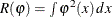 .
.
PROC KDE solves this equation by first evaluating it on a grid of values spaced equally on a log scale. The largest two values from this grid that bound a solution are then used as starting values for a bisection algorithm.
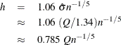
The simple normal reference rule works by assuming  is Gaussian in the preceding fixed-point equation. This results in
![\begin{eqnarray*} h & =& {\hat\sigma } [4/(3n)]^{1/5} \\ & =& 1.06 \ {\hat\sigma } n^{-1/5} \end{eqnarray*}](images/statug_kde0100.png)
where  is the sample standard deviation.
Alternatively, the bandwidth can be computed using the interquartile range, Q:
Silverman’s rule of thumb (Silverman 1986, Section 3.4.2) is computed as
![\[ h = 0.9 \min [{\hat\sigma }, Q/1.34] n^{-1/5} \]](images/statug_kde0103.png)
The oversmoothed bandwidth is computed as
![\[ h = 3{\hat\sigma } [1/(70 \sqrt {\pi } n)]^{1/5} \]](images/statug_kde0104.png)
When you specify a WEIGHT variable, PROC KDE uses weighted versions of  ,
,  , and in the preceding expressions. The weighted quartiles are computed as weighted order statistics, and the weighted variance
takes the form
, and in the preceding expressions. The weighted quartiles are computed as weighted order statistics, and the weighted variance
takes the form
![\[ {\hat\sigma }^{2}=\frac{\sum _{i=1}^{n} W_{i}(X_{i}-\bar{X})^{2}}{\sum _{i=1}^{n} W_{i}} \]](images/statug_kde0107.png)
where  is the weighted sample mean.
For the bivariate case, Wand and Jones (1993) note that automatic bandwidth selection is both difficult and computationally expensive. Their study of various ways of specifying a bandwidth matrix also shows that using two bandwidths, one in each coordinate’s direction, is often adequate. PROC KDE enables you to adjust the two bandwidths by specifying a multiplier for the default bandwidths recommended by Bowman and Foster (1993):
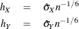
Here  and
and  are the sample standard deviations of X and Y, respectively. These are the optimal bandwidths for two independent normal variables that have the same variances as X and Y. They are, therefore, conservative in the sense that they tend to oversmooth the surface.
You can specify the BWM= option to adjust the aforementioned bandwidths to provide the appropriate amount of smoothing for your application.