The HPQUANTSELECT Procedure

Statistical Tests for Significance Level
The HPQUANTSELECT procedure supports the significance level (SL) criterion for effect selection. Consider the general form of a linear quantile regression model:
![\[ Q_ Y(\tau |\mb{x}_1,\mb{x}_2)=\mb{x}_1’\bbeta _1(\tau )+\mb{x}_2’\bbeta _2(\tau ) \]](images/statug_hpqtr0107.png)
At each step of an effect-selection process, a candidate effect can be represented as  , and the significance level of the candidate effect can be calculated by testing the null hypothesis:
  .
.
When you use SL as a criterion for effect selection, you can further use the TEST= option in the SELECTION statement to specify a statistical test method to compute the significance-level values as follows:
-
The TEST=WALD option specifies the Wald test. Let
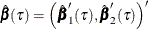 be the parameter estimates for the extended model, and denote the estimated covariance matrix of
  as
as
![\[ \hat{\Sigma }(\tau )=\left[ \begin{array}{cc} \hat{\Sigma }_{11}(\tau )& \hat{\Sigma }_{12}(\tau )\\ \hat{\Sigma }_{21}(\tau )& \hat{\Sigma }_{22}(\tau ) \end{array} \right] \]](images/statug_hpqtr0111.png)
where
 is the covariance matrix for
  . Then the Wald test score is defined as
![\[ \hat{\bbeta }’_2(\tau )\hat{\Sigma }_{22}^{-1}(\tau )\hat{\bbeta }_2(\tau ) \]](images/statug_hpqtr0114.png)
If you specify the SPARSITY(IID) option in the MODEL statement,
 is estimated under the iid errors assumption. Otherwise, is estimated by using non-iid settings. For more information about the linear model with iid errors and non-iid settings,
see the section Quantile Regression.
is estimated under the iid errors assumption. Otherwise, is estimated by using non-iid settings. For more information about the linear model with iid errors and non-iid settings,
see the section Quantile Regression.
-
The TEST=LR1 or TEST=LR2 option specifies the Type I or Type II quasi-likelihood ratio test, respectively. Under the iid assumption, Koenker and Machado (1999) propose two types of quasi-likelihood ratio tests for quantile regression, where the error distribution is flexible but not limited to the asymmetric Laplace distribution. The Type I test score, LR1, is defined as
![\[ {2(D_1(\tau )-D_2(\tau ))\over \tau (1-\tau )\hat{s}} \]](images/statug_hpqtr0116.png)
where
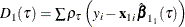 is the sum of check losses for the reduced model,
 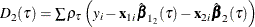 is the sum of check losses for the extended model, and
  is the estimated sparsity function. The Type II test score, LR2, is defined as
![\[ {2D_2(\tau )\left(\log (D_1(\tau ))-\log (D_2(\tau ))\right)\over \tau (1-\tau )\hat{s}} \]](images/statug_hpqtr0120.png)
Under the null hypothesis that the reduced model is the true model, the Wald score, LR1 score, and LR2 score all follow a
 distribution with degrees of freedom
  , where
  and
and  are the degrees of freedom for the reduced model and the extended model, respectively .
When you use SL as a criterion for effect selection, the algorithm for estimating sparsity function depends on whether an
effect is being considered as an add or a drop candidate. For testing an add candidate effect, the sparsity function, which
is  under the iid error assumption or
  for non-iid settings, is estimated on the reduced model that does not include the add candidate effect. For testing a drop
candidate effect, the sparsity function is estimated on the extended model that does not exclude the drop candidate effect.
Then, these estimated sparsity function values are used to compute LR1 or LR2 and the covariance matrix of the parameter estimates
for the extended model. However, for the model that is selected at each step, the sparsity function for estimating standard
errors and confidence limits of the parameter estimates is estimated on that model itself, but not on the model that was selected
at the preceding step.
for non-iid settings, is estimated on the reduced model that does not include the add candidate effect. For testing a drop
candidate effect, the sparsity function is estimated on the extended model that does not exclude the drop candidate effect.
Then, these estimated sparsity function values are used to compute LR1 or LR2 and the covariance matrix of the parameter estimates
for the extended model. However, for the model that is selected at each step, the sparsity function for estimating standard
errors and confidence limits of the parameter estimates is estimated on that model itself, but not on the model that was selected
at the preceding step.
Because the null hypotheses usually do not hold, the SLENTRY and SLSTAY values cannot reliably be viewed as probabilities. One way to address this difficulty is to replace hypothesis testing as a means of selecting a model with information criteria or out-of-sample prediction criteria.
Table 59.6 provides formulas and definitions for these fit statistics.
Table 59.6: Formulas and Definitions for Model Fit Summary Statistics for Single Quantile Effect Selection
|
Statistic |
Definition or Formula |
|---|---|
|
n |
Number of observations |
|
p |
Number of parameters, including the intercept |
|
|
Residual for the ith observation; |
|
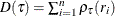
|
Total sum of check losses; |
|
|
Total sum of check losses for intercept-only model if the intercept is a forced-in effect; otherwise for empty model. |
|
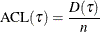
|
Average check loss; |
|
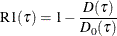
|
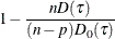
Counterpart of linear regression R square for quantile regression; |
|
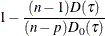
|
Adjusted R1; |
|
|
|
|
|
|
|
|
|


The  criterion is equivalent to the generalized approximate cross validation (GACV) criterion for quantile regression (Yuan 2006). The GACV criterion is defined as
![\[ \mbox{GACV}(\tau )=D(\tau )/ (n-p) \]](images/statug_hpqtr0143.png)
which is proportional to  .
.