The GLMSELECT Procedure
-
Overview

- Getting Started
-
Syntax
-
DetailsModel-Selection MethodsModel Selection IssuesCriteria Used in Model Selection MethodsCLASS Variable Parameterization and the SPLIT OptionMacro Variables Containing Selected ModelsUsing the STORE StatementBuilding the SSCP MatrixModel AveragingUsing Validation and Test DataCross ValidationExternal Cross ValidationScreeningDisplayed OutputODS Table NamesODS Graphics
-
Examples
- References
Example 49.8 Group LASSO Selection
This example shows how you can use the group LASSO method for model selection. This example treats the parameters that correspond to the same spline and CLASS variable as a group and also uses a collection effect to group otherwise unrelated parameters. The following DATA step generates the data:
%macro makeRegressorData(data=,nObs=500,nCont=5,nClass=5,nLev=3);
   data &data;
      drop i j;
      %if &nCont>0  %then %do; array x{&nCont}  x1-x&nCont; %end;
      %if &nClass>0 %then %do; array c{&nClass} c1-c&nClass;%end;
      do i = 1 to &nObs;
         %if &nCont>0 %then %do;
            do j= 1 to &nCont;
               x{j} = rannor(1);
            end;
         %end;
         %if &nClass > 0 %then %do;
            do j=1 to &nClass;
               if      mod(j,3) = 0 then c{j} = ranbin(1,&nLev,.6);
               else if mod(j,3) = 1 then c{j} = ranbin(1,&nLev,.5);
               else if mod(j,3) = 2 then c{j} = ranbin(1,&nLev,.4);
            end;
         %end;
         output;
      end;
   run;
%mend;
%makeRegressorData(data=traindata,nObs=500,nCont=5,nClass=5,nLev=3);
In the generated data, there are five continuous effects, x1–x5, and five CLASS variables, c1–c5. The following DATA step generates a response, y, that is dependent on x1–x4 and c1:
%macro AddDepVar(data=,modelRHS =,errorStd = 1);
   data &data;
      set &data;
      y = &modelRHS + &errorStd * rannor(1);
   run;
%mend;

%AddDepVar(data    = traindata,
           modelRHS= x1 +
                     0.1*x2 - 0.1*x3 - 0.01* x4 -
                     c1,
           errorStd= 1);
The effects x1 and c1 have a stronger influence on the response y than x2 and x3, and x4 has the weakest influence. For the continuous effect x1, a spline effect is constructed using the cubic B-spline basis (see the section EFFECT Statement in Chapter 19: Shared Concepts and Topics) as follows:
effect s1=spline(x1)
Models that contain spline effects are particularly good candidates for group LASSO selection, because the individual parameters in a spline effect have no meaning by themselves. You need them all to be in the model together in order to define the correct spline term in the model.
To have a basis for comparison, first use the following statements to apply LASSO to model selection:
ods graphics on;

proc glmselect data=traindata plots=coefficients;
  class c1-c5/split;
  effect s1=spline(x1/split);
  model y = s1 x2-x5 c:/
        selection=lasso(steps=20 choose=sbc);
run;
In LASSO selection, effects that have multiple parameters are split into their constituent parameters. In this problem, the
spline effect has seven parameters by default and each of the five CLASS effects has four parameters. So together with the
intercept and four continuous main effects, your model has a total of 32 parameters, as shown in the "Dimensions" table in
Output 49.8.1. Note that the number of effects in the table is 17, because the spline effect s1 is counted as 7 effects.
Output 49.8.1: Dimensions
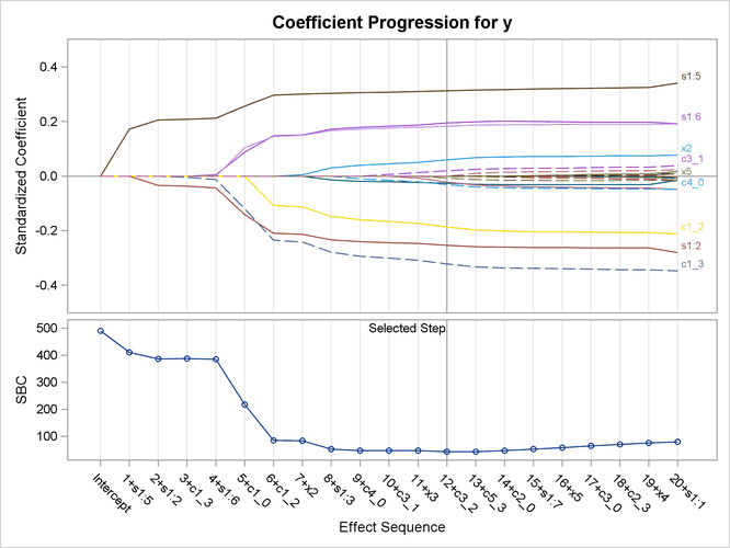
Output 49.8.2 shows the "LASSO Selection Summary" table, and Output 49.8.3 shows the standardized coefficients of all the effects selected at some step of the LASSO method, plotted as a function of
the step number. Because you specified CHOOSE=SBC to pick the best model, the SBC value for the model at each step is also
displayed in Output 49.8.3, with the minimum occurring at step 12. Hence the model at this step is selected, resulting in 13 selected effects. The "Parameter
Estimates" table in Output 49.8.4 shows that x2 and x3 as well as parts of the spline effect and parts of three CLASS effects are selected for the final model. So this selection
misses the small true effect of x4 and erroneously includes c3 and c4 because of noise.
Output 49.8.2: LASSO Selection Summary Table
| The GLMSELECT Procedure |
| LASSO Selection Summary |
| Step | Effect Entered |
Effect Removed |
Number Effects In |
SBC |
|---|---|---|---|---|
| 0 | Intercept | 1 | 491.1109 | |
| 1 | s1:5 | 2 | 410.2008 | |
| 2 | s1:2 | 3 | 386.7278 | |
| 3 | c1_3 | 4 | 388.1524 | |
| 4 | s1:6 | 5 | 385.0045 | |
| 5 | c1_0 | 6 | 216.9169 | |
| 6 | c1_2 | 7 | 84.3459 | |
| 7 | x2 | 8 | 82.8547 | |
| 8 | s1:3 | 9 | 52.3145 | |
| 9 | c4_0 | 10 | 46.8144 | |
| 10 | c3_1 | 11 | 46.6228 | |
| 11 | x3 | 12 | 46.2866 | |
| 12 | c3_2 | 13 | 42.7335* | |
| 13 | c5_3 | 14 | 42.8659 | |
| 14 | c2_0 | 15 | 47.1151 | |
| 15 | s1:7 | 16 | 52.5826 | |
| 16 | x5 | 17 | 58.3346 | |
| 17 | c3_0 | 18 | 63.8812 | |
| 18 | c2_3 | 19 | 69.4954 | |
| 19 | x4 | 20 | 75.6385 | |
| 20 | s1:1 | 21 | 79.8007 | |
| * Optimal Value of Criterion | ||||
Output 49.8.3: LASSO Coefficient Progression Plot
Output 49.8.4: LASSO Parameter Estimates
As opposed to what happens in LASSO selection, spline effects and classification effects are not split by default in group LASSO selection. In addition, you can use a collection effect to construct a group of three of the continuous effects, as shown in the following statements:
proc glmselect data=traindata plots=coefficients;
  class c1-c5;
  effect s1=spline(x1);
  effect s2=collection(x2 x3 x4);
  model y = s1 s2 x5 c:/
        selection=grouplasso(steps=20 choose=sbc rho=0.8);
run;
Because spline and classification effects are not split by default in group LASSO selection, this model contains nine effects:
s1, s2, x5, c1–c5, and the intercept. The number of parameters is the same as before, as shown in Output 49.8.5.
Output 49.8.5: Dimensions
The RHO=0.8 option specifies the value of  for determining the regularization parameter
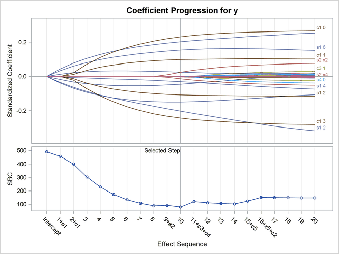
  used in the ith step of the group LASSO selection process. If you use a larger value for , you can expect the plot shown in Output 49.8.7 to exhibit a finer coefficient progression.
Output 49.8.6 shows the "Group LASSO Selection Summary" table, and Output 49.8.7 shows the standardized coefficients of all the effects selected at some step of the group LASSO method, plotted as a function of the step number. As you can see in this plot, the CHOOSE=SBC option selects the model at step 10 as the one that has the minimum value of the SBC statistic. The resulting model contains the four effects, including all the true ones, and 15 parameters, as shown in the "Parameter Estimates" table in Output 49.8.8.
Unlike LASSO, which adds or drops an effect at each step, the group LASSO method can add or drop more than one effect. Indeed, you can see in Output 49.8.7 that steps 11 and 16 each added two effects to the model. Simple selection breaks down because group LASSO does not admit a piecewise linear constant solution path, as regular LASSO does.
Output 49.8.6: Group LASSO Selection Summary Table
| The GLMSELECT Procedure |
| Group LASSO Selection Summary |
| Step | Effect Entered |
Effect Removed |
Number Effects In |
SBC |
|---|---|---|---|---|
| 0 | Intercept | 1 | 491.1109 | |
| 1 | s1 | 2 | 457.0038 | |
| 2 | c1 | 3 | 400.1165 | |
| 3 | 3 | 302.8975 | ||
| 4 | 3 | 228.2883 | ||
| 5 | 3 | 173.3913 | ||
| 6 | 3 | 134.3346 | ||
| 7 | 3 | 107.2038 | ||
| 8 | 3 | 88.6178 | ||
| 9 | s2 | 4 | 91.9567 | |
| 10 | 4 | 79.7022* | ||
| 11 | c3 c4 | 6 | 119.8826 | |
| 12 | 6 | 111.5926 | ||
| 13 | 6 | 105.8915 | ||
| 14 | 6 | 101.9617 | ||
| 15 | c5 | 7 | 123.6787 | |
| 16 | x5 c2 | 9 | 152.2387 | |
| 17 | 9 | 150.4210 | ||
| 18 | 9 | 149.1847 | ||
| 19 | 9 | 148.3496 | ||
| 20 | 9 | 147.7893 | ||
| * Optimal Value of Criterion | ||||
Output 49.8.7: LASSO Coefficient Progression Plot
Output 49.8.8: Group LASSO Parameter Estimates