The GLMPOWER Procedure

Example 48.3 Repeated Measures ANOVA
Logan, Baron, and Kohout (1995) and Guo et al. (2013) study the effect of a dental intervention on the memory of pain after root canal therapy. The intervention is a sensory focus strategy, in which patients are instructed to pay attention only to the physical sensations in their mouth during the root canal procedure.
Suppose you are interested in the long-term effects of this sensory focus intervention, because avoidance behavior has been shown to build along with memory of pain. You are planning a study to compare sensory focus to standard of care over a period of a year, asking patients to self-report their memory of pain immediately after the procedure and then again at 1 week, 6 months, and 12 months. You use a scale from 0 (no pain remembered) to 5 (maximum pain remembered).
The between-subject factor in your model is treatment, with two levels (sensory focus versus standard of care), and you allocate each treatment equally for a balanced design. The within-subject factor is time, with four levels (0, 1, 26, and 52 weeks).
You want to determine the number of patients who are needed in order to achieve a power of 0.9 at significance level  = 0.01 for the test of the interaction between time and treatment, where the contrast over time contains all pairwise comparisons.
You also want to generate a plot of power versus sample size that covers the power range of 0.05 to 0.99.
= 0.01 for the test of the interaction between time and treatment, where the contrast over time contains all pairwise comparisons.
You also want to generate a plot of power versus sample size that covers the power range of 0.05 to 0.99.
The default Hotelling-Lawley F test is appropriate for this study, especially because it is the same as the Wald test in PROC MIXED with the DDFM=KR Kenward-Roger degrees-of-freedom method and an unstructured covariance model.
You conjecture that the mean memory of pain for each treatment follows the information in Table 48.13.
Table 48.13: Mean Memory of Pain by Treatment
|
Time Since Root Canal Therapy |
||||
|---|---|---|---|---|
|
Treatment |
Later on Same Day |
1 Week |
6 Months |
12 Months |
|
Sensory Focus |
2.40 |
2.38 |
2.05 |
1.90 |
|
Standard of Care |
2.40 |
2.39 |
2.36 |
2.30 |
The following statements create a data set named Pain that is to contain these means over treatment and time:
data Pain;
   input Treatment $ PainMem0 PainMem1Wk PainMem6Mo PainMem12Mo;
   datalines;
      SensoryFocus    2.40  2.38  2.05  1.90
      StandardOfCare  2.40  2.39  2.36  2.30
;
The variable Treatment specifies the two treatments. The four variables PainMem0, PainMem1Wk, PainMem6Mo, and PainMem12Mo specify the mean memory of pain scores in Table 48.13.
To characterize the variability, you must specify a set of parameters that defines the entire covariance matrix of the residuals. You conjecture that the error standard deviation is the same at all four time points, with a value somewhere between 0.92 and 1.04, and you account for your uncertainty by including both the lower and upper ends of this range in the sample size analysis. You believe that the correlation has a linear exponent autoregressive (LEAR) structure, with a correlation of about 0.6 between measurements one week apart and a decay rate of about 0.8 over one-week intervals. The correlation matrix that contains these LEAR parameters, rounded to three decimal places, is shown in Table 48.14.
Table 48.14: Conjectured Correlation Matrix
|
|
0 |
1 |
26 |
52 |
|
0 |
1 |
0.6 |
0.491 |
0.399 |
|
1 |
0.6 |
1 |
0.495 |
0.402 |
|
26 |
0.491 |
0.495 |
1 |
0.491 |
|
52 |
0.399 |
0.402 |
0.491 |
1 |
Use the DATA=
option in the PROC GLMPOWER
statement to specify Pain as the exemplary data set. Specify the between- and within-subject factors and the model by using the CLASS
, MODEL
, and REPEATED
statements just as you would in PROC GLM for the repeated measures data analysis. Use the POWER
statement to indicate sample size as the result parameter and specify the other analysis parameters, and use the PLOT
statement to generate the power curves. The following statements perform the sample size analysis:
ods graphics on;
proc glmpower data=Pain;
class Treatment;
model PainMem0 PainMem1Wk PainMem6Mo PainMem12Mo = Treatment;
repeated Time contrast;
power
mtest = hlt
alpha = 0.01
power = .9
ntotal = .
stddev = 0.92 1.04
matrix ("PainCorr") = lear(0.6, 0.8, 4, 0 1 26 52)
corrmat = "PainCorr";
plot y=power min=0.05 max=0.99 yopts=(ref=0.9)
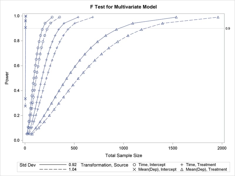
vary (linestyle by stddev, symbol by dependent source);
run;
ods graphics off;
The STDDEV= option specifies the two scenarios for the common residual standard deviation, 0.92 and 1.04. The MATRIX= option defines the LEAR correlation structure, and the CORRMAT= option specifies it as the correlation matrix of the residuals. The Y= POWER option in the PLOT statement requests a plot that has power on the Y axis. (The result parameter—in this case, total sample size—is always plotted on the other axis.) The MIN= and MAX= options in the PLOT statement specify the power range. The YOPTS= (REF= ) option adds a reference line at the target power value of 0.9. The VARY option specifies that the line style vary by the residual standard deviation and that the plotting symbol vary by the combination of within-subject and between-subject effects. The ODS GRAPHICS ON statement enables ODS Graphics.
Output 48.3.1 shows the output, and Output 48.3.2 shows the plot.
Output 48.3.1: Sample Size Analysis for Repeated Measures
| Computed N Total | ||||||||
|---|---|---|---|---|---|---|---|---|
| Index | Transformation | Source | Std Dev | Effect | Num DF | Den DF | Actual Power | N Total |
| 1 | Time | Intercept | 0.92 | Time | 3 | 176 | 0.900 | 180 |
| 2 | Time | Intercept | 1.04 | Time | 3 | 226 | 0.903 | 230 |
| 3 | Time | Treatment | 0.92 | Time*Treatment | 3 | 346 | 0.901 | 350 |
| 4 | Time | Treatment | 1.04 | Time*Treatment | 3 | 442 | 0.901 | 446 |
| 5 | Mean(Dep) | Intercept | 0.92 | Intercept | 1 | 4 | 0.960 | 6 |
| 6 | Mean(Dep) | Intercept | 1.04 | Intercept | 1 | 4 | 0.907 | 6 |
| 7 | Mean(Dep) | Treatment | 0.92 | Treatment | 1 | 950 | 0.900 | 952 |
| 8 | Mean(Dep) | Treatment | 1.04 | Treatment | 1 | 1214 | 0.900 | 1216 |
Output 48.3.1 reveals that the required sample size to achieve a power of 0.9 for the test of the Time*Treatment interaction is 350 for the error standard deviation of 0.92 and 446 for the error standard deviation of 1.04.
Output 48.3.2: Plot of Power versus Sample Size for Repeated Measures Analysis