The FMM Procedure

PROC FMM Statement
-
PROC FMM <options>;
The PROC FMM statement invokes the FMM procedure. Table 39.2 summarizes the options available in the PROC FMM statement. These and other options in the PROC FMM statement are then described fully in alphabetical order.
Table 39.2: PROC FMM Statement Options
|
Option |
Description |
|---|---|
|
Basic Options |
|
|
Specifies the input data set |
|
|
Specifies how the procedure responds to support violations in the data |
|
|
Specifies the length of effect names |
|
|
Determines the sort order of CLASS variables |
|
|
Specifies the random number seed for analyses that require random number draws |
|
|
Displayed Output |
|
|
Displays information about the mixture components |
|
|
Displays the asymptotic correlation matrix of the maximum likelihood parameter estimates or the empirical correlation matrix of the Bayesian posterior estimates |
|
|
Displays the asymptotic covariance matrix of the maximum likelihood parameter estimates or the empirical covariance matrix of the Bayesian posterior estimates |
|
|
Displays the inverse of the covariance matrix of the parameter estimates |
|
|
Displays fit information for all examined models |
|
|
Adds estimates and gradients to the "Iteration History" table |
|
|
Suppresses the "Class Level Information" table completely or partially |
|
|
Suppresses the "Iteration History Information" table |
|
|
Suppresses tabular and graphical output |
|
|
Specifies how parameters are displayed in ODS tables |
|
|
Produces ODS statistical graphics |
|
|
Computational Options |
|
|
Specifies the criterion used in model selection |
|
|
Prevents centering and scaling of the regressor variables |
|
|
Specifies a variable that defines a partial classification |
|
|
Options Related to Optimization |
|
|
Tunes an absolute function convergence criterion |
|
|
Tunes an absolute function difference convergence criterion |
|
|
Tunes the absolute gradient convergence criterion |
|
|
Specifies a relative function convergence criterion that is based on a relative change of the function value |
|
|
Specifies a relative function convergence criterion that is based on a predicted reduction of the objective function |
|
|
Tunes the relative gradient convergence criterion |
|
|
Specifies the maximum number of iterations in any optimization |
|
|
Specifies the maximum number of function evaluations in any optimization |
|
|
Specifies the upper limit of CPU time in seconds for any optimization |
|
|
Specifies the minimum number of iterations in any optimization |
|
|
Selects the optimization technique |
|
|
Singularity Tolerances |
|
|
Tunes the value assigned to an invalid component log likelihood |
|
|
Tunes singularity for Cholesky decompositions |
|
|
Tunes singularity for the residual variance |
|
|
Tunes general singularity criterion |
|
|
Tunes component weight threshold for number of effective components |
|
You can specify the following options in the PROC FMM statement.
-
ABSCONV=r
ABSTOL=r -
specifies an absolute function convergence criterion. For minimization, the termination criterion is
 , where
  is the vector of parameters in the optimization and
  is the objective function. The default value of r is the negative square root of the largest double-precision value, which serves only as a protection against overflows.
-
ABSFCONV=r <n>
ABSFTOL=r<n> -
specifies an absolute function difference convergence criterion. For all techniques except NMSIMP, the termination criterion is a small change of the function value in successive iterations:
![\[ |f(\bpsi ^{(k-1)}) - f(\bpsi ^{(k)})| \leq r \]](images/statug_fmm0031.png)
Here,
denotes the vector of parameters that participate in the optimization, and is the objective function. The same formula is used for the NMSIMP technique, but  is defined as the vertex with the lowest function value, and
  is defined as the vertex with the highest function value in the simplex. The default value is r=0. The optional integer value n specifies the number of successive iterations for which the criterion must be satisfied before the process can be terminated.
-
ABSGCONV=r <n>
ABSGTOL=r<n> -
specifies an absolute gradient convergence criterion. The termination criterion is a small maximum absolute gradient element:
![\[ \max _ j |g_ j(\bpsi ^{(k)})| \leq r \]](images/statug_fmm0034.png)
Here,
denotes the vector of parameters that participate in the optimization, and  is the gradient of the objective function with respect to the jth parameter. This criterion is not used by the NMSIMP technique. The default value is r=1E–5. The optional integer value n specifies the number of successive iterations for which the criterion must be satisfied before the process can be terminated.
-
COMPONENTINFO
COMPINFO
CINFO -
produces a table with additional details about the fitted model components.
- COV
-
produces the covariance matrix of the parameter estimates. For maximum likelihood estimation, this matrix is based on the inverse (projected) Hessian matrix. For Bayesian estimation, it is the empirical covariance matrix of the posterior estimates. The covariance matrix is shown for all parameters, even if they did not participate in the optimization or sampling.
- COVI
-
produces the inverse of the covariance matrix of the parameter estimates. For maximum likelihood estimation, the covariance matrix is based on the inverse (projected) Hessian matrix. For Bayesian estimation, it is the empirical covariance matrix of the posterior estimates. This matrix is then inverted by sweeping, and rows and columns that correspond to linear dependencies or singularities are zeroed.
- CORR
-
produces the correlation matrix of the parameter estimates. For maximum likelihood estimation this matrix is based on the inverse (projected) Hessian matrix. For Bayesian estimation, it is based on the empirical covariance matrix of the posterior estimates.
-
CRITERION=keyword
CRIT=keyword -
specifies the criterion by which the FMM procedure ranks models when multiple models are evaluated during maximum likelihood estimation. You can choose from the following criteria to rank models by specifying the appropriate keyword:
- AIC
-
uses Akaike’s information criterion.
- AICC
-
uses the bias-corrected AIC criterion.
- BIC
-
uses the Bayesian information criterion.
- GRADIENT
-
uses the largest element of the gradient (in absolute value).
- LOGL | LL
-
uses the mixture log likelihood.
- PEARSON
-
uses the Pearson statistic.
The default for maximum likelihood estimation is CRITERION=BIC.
In Bayesian model selection, you can choose from the following criteria to rank models:
- DIC
-
uses the deviance information criterion.
- LOGL | LL
-
uses the mixture log likelihood
The default for Bayesian estimation is CRITERION=DIC.
- DATA=SAS-data-set
-
names the SAS data set to be used by PROC FMM. The default is the most recently created data set.
-
EXCLUSION=NONE | ANY | ALL
EXCLUDE=NONE | ANY | ALL -
specifies how the FMM procedure handles support violations of observations. For example, in a mixture of two Poisson variables, negative response values are not possible. However, in a mixture of a Poisson and a normal variable, negative values are possible, and their likelihood contribution to the Poisson component is zero. An observation that violates the support of one component distribution of the model might be a valid response with respect to one or more other component distributions. This requires some nuanced handling of support violations in mixture models.
The default exclusion technique, EXCLUSION=ALL, removes an observation from the analysis only if it violates the support of all component distributions. The other extreme, EXCLUSION=NONE, permits an observation into the analysis regardless of support violations. EXCLUSION=ANY removes observations from the analysis if the response violates the support of any component distributions. In the single-component case, EXCLUSION=ALL and EXCLUSION=ANY are identical.
-
FCONV=r<n>
FTOL=r<n> -
specifies a relative function convergence criterion that is based on the relative change of the function value. For all techniques except NMSIMP, PROC FMM terminates when there is a small relative change of the function value in successive iterations:
![\[ \frac{|f(\bpsi ^{(k)}) - f(\bpsi ^{(k-1)})|}{|f(\bpsi ^{(k-1)})|} \leq r \]](images/statug_fmm0036.png)
Here,
denotes the vector of parameters that participate in the optimization, and is the objective function. The same formula is used for the NMSIMP technique, but  is defined as the vertex with the lowest function value, and is defined as the vertex with the highest function value in the simplex.
The default is
 , where FDIGITS is by default
  , and
, and  is the machine precision. The optional integer value n specifies the number of successive iterations for which the criterion must be satisfied before the process terminates.
-
FCONV2=r<n>
FTOL2=r<n> -
specifies a relative function convergence criterion that is based on the predicted reduction of the objective function. For all techniques except NMSIMP, the termination criterion is a small predicted reduction
![\[ df^{(k)} \approx f(\btheta ^{(k)}) - f(\btheta ^{(k)} + \mb{s}^{(k)}) \]](images/statug_fmm0041.png)
of the objective function. The predicted reduction
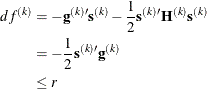
is computed by approximating the objective function f by the first two terms of the Taylor series and substituting the Newton step:
![\[ \mb{s}^{(k)} = - [\mb{H}^{(k)}]^{-1} \mb{g}^{(k)} \]](images/statug_fmm0043.png)
For the NMSIMP technique, the termination criterion is a small standard deviation of the function values of the
 simplex vertices
  ,
,  ,
,
![\[ \sqrt { \frac{1}{n+1} \sum _ l \left[ f(\btheta _ l^{(k)}) - \overline{f}(\btheta ^{(k)}) \right]^2 } \leq r \]](images/statug_fmm0047.png)
where
 . If there are
  boundary constraints active at
  , the mean and standard deviation are computed only for the
  unconstrained vertices.
The default value is r = 1E–6 for the NMSIMP technique and r = 0 otherwise. The optional integer value n specifies the number of successive iterations for which the criterion must be satisfied before the process terminates.
- FITDETAILS
-
requests that the "Optimization Information," "Iteration History," "Convergence Status," and "Fit Statistics" tables be produced for all optimizations when models with different number of components are evaluated. For example, the following statements fit a binomial regression model with up to three components and produces fit and optimization information for all three:
proc fmm fitdetails;
   model y/n  = x / kmax=3;
run;
Without the FITDETAILS option, only the "Fit Statistics" table for the selected model is displayed.
In Bayesian estimation, the FITDETAILS option displays the following tables for each model that the procedure fits: "Bayes Information," "Iteration History," "Prior Information," "Fit Statistics," "Posterior Summaries," "Posterior Intervals," and any requested diagnostics tables. The "Iteration History" table appears only if the BAYES statement includes the INITIAL= MLE option.
Without the FITDETAILS option, these tables are listed only for the selected model.
-
GCONV=r<n>
GTOL=r<n> -
specifies a relative gradient convergence criterion. For all techniques except CONGRA and NMSIMP, the termination criterion is a small normalized predicted function reduction:
![\[ \frac{\mb{g}(\bpsi ^{(k)})^\prime [\bH ^{(k)}]^{-1} \mb{g}(\bpsi ^{(k)})}{|f(\bpsi ^{(k)})| } \leq r \]](images/statug_fmm0052.png)
Here,
denotes the vector of parameters that participate in the optimization, is the objective function, and  is the gradient. For the CONGRA technique (where a reliable Hessian estimate
  is not available), the following criterion is used:
![\[ \frac{\parallel \mb{g}(\bpsi ^{(k)}) \parallel _2^2 \quad \parallel \mb{s}(\bpsi ^{(k)}) \parallel _2}{\parallel \mb{g}(\bpsi ^{(k)}) - \mb{g}(\bpsi ^{(k-1)}) \parallel _2 |f(\bpsi ^{(k)})| } \leq r \]](images/statug_fmm0055.png)
This criterion is not used by the NMSIMP technique. The default value is r = 1E–8. The optional integer value n specifies the number of successive iterations for which the criterion must be satisfied before the process can terminate.
- HESSIAN
-
displays the Hessian matrix of the model. This option is not available for Bayesian estimation.
- INVALIDLOGL=r
-
specifies the value assumed by the FMM procedure if a log likelihood cannot be computed (for example, because the value of the response variable falls outside of the response distribution’s support). The default value is –1E20.
- ITDETAILS
-
adds parameter estimates and gradients to the "Iteration History" table. If the FMM procedure centers or scales the model variables (or both), the parameter estimates and gradients reported during the iteration refer to that scale. You can suppress centering and scaling with the NOCENTER option.
-
MAXFUNC=n
MAXFU=n -
specifies the maximum number of function calls in the optimization process. The default values are as follows, depending on the optimization technique:
-
TRUREG, NRRIDG, and NEWRAP: 125
-
QUANEW and DBLDOG: 500
-
CONGRA: 1000
-
NMSIMP: 3000
The optimization can terminate only after completing a full iteration. Therefore, the number of function calls that are actually performed can exceed the number that is specified by the MAXFUNC= option. You can choose the optimization technique with the TECHNIQUE= option.
-
-
MAXITER=n
MAXIT=n -
specifies the maximum number of iterations in the optimization process. The default values are as follows, depending on the optimization technique:
-
TRUREG, NRRIDG, and NEWRAP: 50
-
QUANEW and DBLDOG: 200
-
CONGRA: 400
-
NMSIMP: 1000
These default values also apply when n is specified as a missing value. You can choose the optimization technique with the TECHNIQUE= option.
-
- MAXTIME=r
-
specifies an upper limit of r seconds of CPU time for the optimization process. The time is checked only at the end of each iteration. Therefore, the actual run time might be longer than the specified time. By default, CPU time is not limited.
-
MINITER=n
MINIT=n -
specifies the minimum number of iterations. The default value is 0. If you request more iterations than are actually needed for convergence to a stationary point, the optimization algorithms can behave strangely. For example, the effect of rounding errors can prevent the algorithm from continuing for the required number of iterations.
- NAMELEN=number
-
specifies the length to which long effect names are shortened. The default and minimum value is 20.
- NOCENTER
-
requests that regressor variables not be centered or scaled. By default the FMM procedure centers and scales columns of the
 matrix if the models contain intercepts. If NOINT
options in MODEL
statements are in effect, the columns of are scaled but not centered. Centering and scaling can help with the stability of estimation and sampling algorithms. The
FMM procedure does not produce a table of the centered and scaled coefficients and provides no user control over the type
of centering and scaling that is applied. The NOCENTER option turns any centering and scaling off and processes the raw values
of the continuous variables.
matrix if the models contain intercepts. If NOINT
options in MODEL
statements are in effect, the columns of are scaled but not centered. Centering and scaling can help with the stability of estimation and sampling algorithms. The
FMM procedure does not produce a table of the centered and scaled coefficients and provides no user control over the type
of centering and scaling that is applied. The NOCENTER option turns any centering and scaling off and processes the raw values
of the continuous variables.
- NOCLPRINT<=number>
-
suppresses the display of the "Class Level Information" table if you do not specify number. If you specify number, the values of the classification variables are displayed for only those variables whose number of levels is less than number. Specifying a number helps to reduce the size of the "Class Level Information" table if some classification variables have a large number of levels.
- NOITPRINT
-
suppresses the display of the "Iteration History Information" table.
- NOPRINT
-
suppresses the normal display of tabular and graphical results. The NOPRINT option is useful when you want to create only one or more output data sets with the procedure. This option temporarily disables the Output Delivery System (ODS); see Chapter 20: Using the Output Delivery System, for more information.
- ORDER=order-type
-
specifies the sort order for the levels of CLASS variables. This ordering determines which parameters in the model correspond to each level in the data.
You can specify the following values for order-type:
When the default ORDER=FORMATTED is in effect for numeric variables for which you have supplied no explicit format, the levels are ordered by their internal values. To order numeric class levels with no explicit format by their BEST12. formatted values, you can specify this format explicitly for the CLASS variables.
When FORMATTED and INTERNAL values are involved, the sort order is machine-dependent.
When the response variable appears in a CLASS statement, the ORDER= option in the PROC FMM statement applies to its sort order. For example, in the following statements the sort order of the
wheezevariable is determined by the order of appearance in the input data set because the response variable appears in the CLASS statement:proc fmm order=data; class city wheeze; model wheeze = city age / dist=binary s; run;
However, in the following statements the sort order of the
wheezevariable is determined by the formatted value (the default response-option in the MODEL statement):proc fmm order=data; class city; model wheeze = city age / dist=binary s; run;
The ORDER= option in the PROC FMM statement has no effect on the sort order of the
wheezevariable because it does not appear in the CLASS statement.When you specify a response-option in the MODEL statement, it overrides the ORDER= option in the PROC FMM statement.
For more information about sort order, see the chapter on the SORT procedure in the Base SAS Procedures Guide and the discussion of BY-group processing in SAS Language Reference: Concepts.
- PARMSTYLE=EFFECT | LABEL
-
specifies the display style for parameters and effects. The FMM procedure can display parameters in two styles:
-
The EFFECT style (which is used by the MIXED and GLIMMIX procedure, for example) identifies a parameter with an "Effect" column and adds separate columns for the CLASS variables in the model.
-
The LABEL style creates one column, named Parameter, that combines the relevant information about a parameter into a single column. If your model contains multiple CLASS variables, the LABEL style might use space more economically.
The EFFECT style is the default for models that contain effects; otherwise the LABEL style is used (for example, in homogeneous mixtures). You can change the display style with the PARMSTYLE= option. Regardless of the display style, ODS output data sets that contain information about parameter estimates contain columns for both styles.
-
-
PARTIAL=variable
MEMBERSHIP=variable -
specifies a variable in the input data set that identifies component membership. You can specify missing values for observations whose component membership is undetermined; this is known as a partial classification (McLachlan and Peel 2000, p. 75). For observations with known membership, the likelihood contribution is no longer a mixture. If observation i is known to be a member of component m, then its log likelihood contribution is
![\[ \log \left\{ \pi _ m(\mb{z},\balpha _ m) \, \, p_ m(y;\mb{x}_ m’\bbeta _ m,\phi _ m)\right\} \]](images/statug_fmm0057.png)
Otherwise, if membership is undetermined, it is
![\[ \log \left\{ \sum _{j=1}^{k} \, \, \pi _ j(\mb{z},\balpha _ j) p_ j(y;\mb{x}_ j’\bbeta _ j,\phi _ j)\right\} \]](images/statug_fmm0058.png)
The
variablespecified in the PARTIAL= option can be numeric or character. In case of a character variable, the variable must appear in the CLASS statement. If the PARTIAL= variable appears in the CLASS statement, the membership assignment is made based on the levelized values of the variable, as shown in the "Class Level Information" table. Invalid values of the PARTIAL= variable are ignored.In a model in which label switching is a problem, the switching can sometimes be avoided by assigning just a few observations to categories. For example, in a three-component model, switches might be prevented by assigning the observation with the smallest response value to the first component and the observation with the largest response value to the last component.
-
PLOTS <(global-plot-options)> <=plot-request <(options)>>
PLOTS <(global-plot-options)> <=(plot-request <(options)> <... plot-request <(options)>>)> -
controls the graphical output that is produced through ODS Graphics.
ODS Graphics must be enabled before plots can be requested. For example:
ods graphics on;
proc fmm data=yeast seed=12345;
   model count/n = / k=2;
   freq f;
   performance cpucount=2;
   bayes;
run;
ods graphics off;
For more information about enabling and disabling ODS Graphics, see the section Enabling and Disabling ODS Graphics in Chapter 21: Statistical Graphics Using ODS.
Global Plot Options
The global-plot-options apply to all relevant plots generated by the FMM procedure. The global-plot-options supported by the FMM procedure are as follows:
Specific Plot Options
The following listing describes the specific plots and their options.
- SEED=n
-
determines the random number seed for analyses that depend on a random number stream. If you do not specify a seed or if you specify a value less than or equal to zero, the seed is generated from reading the time of day from the computer clock. The largest possible value for the seed is
 . The seed value is reported in the "Model Information" table.
You can use the SYSRANDOM and SYSRANEND macro variables after a PROC FMM run to query the initial and final seed values. However, using the final seed value as the starting seed for a subsequent analysis does not continue the random number stream where the previous analysis left off. The SYSRANEND macro variable provides a mechanism to pass on seed values to ensure that the sequence of random numbers is the same every time you run an entire program.
Analyses that use the same (nonzero) seed are not completely reproducible if they are executed with a different number of threads because the random number streams in separate threads are independent. You can control the number of threads used by the FMM procedure with system options or through the PERFORMANCE statement in the FMM procedure.
- SINGCHOL=number
-
tunes the singularity criterion in Cholesky decompositions. The default is 1E4 times the machine epsilon; this product is approximately 1E–12 on most computers.
- SINGRES=number
-
sets the tolerance for which the residual variance or scale parameter is considered to be zero. The default is 1E4 times the machine epsilon; this product is approximately 1E–12 on most computers.
- SINGULAR=number
-
tunes the general singularity criterion applied by the FMM procedure in sweeps and inversions. The default is 1E4 times the machine epsilon; this product is approximately 1E–12 on most computers.
-
TECHNIQUE=keyword
TECH=keyword -
specifies the optimization technique to obtain maximum likelihood estimates. You can choose from the following techniques by specifying the appropriate keyword:
- CONGRA
-
performs a conjugate-gradient optimization.
- DBLDOG
-
performs a version of double-dogleg optimization.
- NEWRAP
-
performs a Newton-Raphson optimization combining a line-search algorithm with ridging.
- NMSIMP
-
performs a Nelder-Mead simplex optimization.
- NONE
-
performs no optimization.
- NRRIDG
-
performs a Newton-Raphson optimization with ridging.
- QUANEW
-
performs a dual quasi-Newton optimization.
- TRUREG
-
performs a trust-region optimization.
The default is TECH=QUANEW.
For more details about these optimization methods, see the section Choosing an Optimization Algorithm in Chapter 19: Shared Concepts and Topics.
- ZEROPROB=number
-
tunes the threshold (a value between 0 and 1) below which the FMM procedure considers a component mixing probability to be zero. This affects the calculation of the number of effective components. The default is the square root of the machine epsilon; this is approximately 1E–8 on most computers.