The BOXPLOT Procedure

Clipping Extreme Values
By default a box plot’s vertical axis is scaled to accommodate all the values in all groups. If the variation between groups is large with respect to the variation within groups, or if some groups contain extreme outlier values, the vertical axis scale can become so large that the box-and-whiskers plots are compressed. In such cases, you can clip the extreme values to produce a more readable plot, as illustrated in the following example.
A company produces copper tubing. The diameter measurements (in millimeters) for 15 batches of five tubes each are provided
in the data set Newtubes:
data Newtubes;
   label Diameter='Diameter in mm';
   do Batch = 1 to 15;
      do  i = 1 to 5;
         input Diameter @@;
         output;
      end;
   end;
   datalines;
69.13  69.83  70.76  69.13  70.81
85.06  82.82  84.79  84.89  86.53
67.67  70.37  68.80  70.65  68.20
71.71  70.46  71.43  69.53  69.28
71.04  71.04  70.29  70.51  71.29
69.01  68.87  69.87  70.05  69.85
50.72  50.49  49.78  50.49  49.69
69.28  71.80  69.80  70.99  70.50
70.76  69.19  70.51  70.59  70.40
70.16  70.07  71.52  70.72  70.31
68.67  70.54  69.50  69.79  70.76
68.78  68.55  69.72  69.62  71.53
70.61  70.75  70.90  71.01  71.53
74.62  56.95  72.29  82.41  57.64
70.54  69.82  70.71  71.05  69.24
;
The following statements create a box plot of the tube diameters:
ods graphics on;
title 'Box Plot for New Copper Tubes' ;
proc boxplot data=Newtubes;
   plot Diameter*Batch / odstitle = title;
run;
The box plot is shown in Figure 28.16.
Figure 28.16: Compressed Box Plots
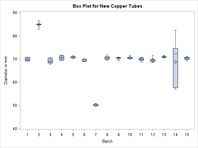
Note that the diameters in batch 2 are significantly larger, and those in batch 7 significantly smaller, than those in most of the other batches. The default vertical axis scaling causes the box-and-whiskers plots to be compressed.
You can produce a more useful box plot by specifying the CLIPFACTOR= factor option, where factor is a value greater than one. Clipping is applied as follows:
-
The mean of the first quartile values (
 ) and the mean of the third quartile values (
 ) are computed across all groups.
-
The following values define the clipping range:
![\[ y_{\max }= \overline{Q1} + ( \overline{Q3} - \overline{Q1} ) \times \mi{factor} \]](images/statug_boxplot0042.png)
and
![\[ y_{\min }= \overline{Q3} - ( \overline{Q3} - \overline{Q1} ) \times \mi{factor} \]](images/statug_boxplot0043.png)
Any statistic greater than
 or less than
  is ignored during vertical axis scaling.
Note:
-
Clipping is applied only to the plotted statistics and not to the statistics saved in an output data set.
-
A special symbol is used for clipped points (the default symbol is a square), and a legend is added to the chart indicating the number of boxes that were clipped.
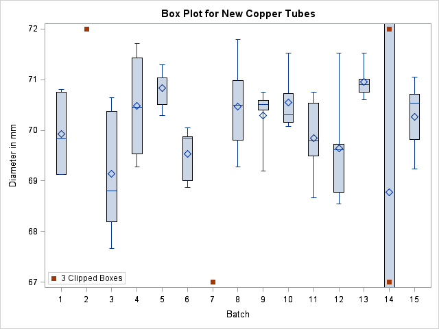
The following statements use a clipping factor of 1.5 to create a box plot of the same data plotted in Figure 28.16:
title 'Box Plot for New Copper Tubes' ;
proc boxplot data=Newtubes;
   plot Diameter*Batch /
      odstitle   = title
      clipfactor = 1.5;
run;
The clipped box plot is shown in Figure 28.17.
Figure 28.17: Box Plot with Clip Factor of 1.5

In Figure 28.17 the extreme values are clipped, making the box plot more readable. The box-and-whiskers plots for batches 2 and 7 are clipped completely, while the plot for batch 14 is clipped at both the top and bottom. Clipped points are marked with a square, and a clipping legend is added at the lower right of the display.
Other clipping options are available, as illustrated by the following statements:
title 'Box Plot for New Copper Tubes' ;
proc boxplot data=Newtubes;
   plot Diameter*Batch /
      odstitle    = title
      clipfactor  = 1.5
      cliplegend  = '# Clipped Boxes'
      clipsubchar = '#';
run;
The CLIPLEGEND= option requests a user-specified legend for the number of clipped boxes. Each occurrence in the legend of the character specified in the CLIPSUBCHAR= option is replaced by the number of clipped boxes.
Figure 28.18 shows the box plot with the modified clipping legend.
Figure 28.18: Box Plot with Clipping Options
For more information about clipping options, see the appropriate entries in the section PLOT Statement Options.