The SEQDESIGN Procedure
-
Overview

- Getting Started
-
Syntax
-
DetailsFixed-Sample Clinical TrialsOne-Sided Fixed-Sample Tests in Clinical TrialsTwo-Sided Fixed-Sample Tests in Clinical TrialsGroup Sequential MethodsStatistical Assumptions for Group Sequential DesignsBoundary ScalesBoundary VariablesType I and Type II ErrorsUnified Family MethodsHaybittle-Peto MethodWhitehead MethodsError Spending MethodsAcceptance (beta) BoundaryBoundary Adjustments for Overlapping Lower and Upper beta BoundariesSpecified and Derived ParametersApplicable Boundary KeysSample Size ComputationApplicable One-Sample Tests and Sample Size ComputationApplicable Two-Sample Tests and Sample Size ComputationApplicable Regression Parameter Tests and Sample Size ComputationAspects of Group Sequential DesignsSummary of Methods in Group Sequential DesignsTable OutputODS Table NamesGraphics OutputODS Graphics
-
ExamplesCreating Fixed-Sample DesignsCreating a One-Sided O’Brien-Fleming DesignCreating Two-Sided Pocock and O’Brien-Fleming DesignsGenerating Graphics Display for Sequential DesignsCreating Designs Using Haybittle-Peto MethodsCreating Designs with Various Stopping CriteriaCreating Whitehead’s Triangular DesignsCreating a One-Sided Error Spending DesignCreating Designs with Various Number of StagesCreating Two-Sided Error Spending Designs with and without Overlapping Lower and Upper beta BoundariesCreating a Two-Sided Asymmetric Error Spending Design with Early Stopping to Reject H0Creating a Two-Sided Asymmetric Error Spending Design with Early Stopping to Reject or Accept H0Creating a Design with a Nonbinding Beta BoundaryComputing Sample Size for Survival Data That Have Uniform AccrualComputing Sample Size for Survival Data with Truncated Exponential Accrual
- References
This example requests a five-stage, one-sided group sequential design for normally distributed statistics. The design uses
an O’Brien-Fleming-type error spending function for the ![]() boundary and a Pocock-type error spending function for the
boundary and a Pocock-type error spending function for the ![]() boundary. The following statements request a one-sided design by using different
boundary. The following statements request a one-sided design by using different ![]() and
and ![]() spending functions:
spending functions:
ods graphics on;
proc seqdesign altref=0.2  errspend
               pss(cref=0 0.5 1)
               stopprob(cref=0 0.5 1)
               plots=(asn power errspend)
               ;
   OneSidedErrorSpending: design nstages=5
                          method(alpha)=errfuncobf
                          method(beta)=errfuncpoc
                          alt=upper  stop=both
                          alpha=0.025
                          ;
run;
ods graphics off;
The "Design Information" table in Output 89.8.1 displays design specifications and the derived statistics. With the specified alternative reference, the maximum information is derived.
Output 89.8.1: Error Spending Method Design Information
| Design Information | |
|---|---|
| Statistic Distribution | Normal |
| Boundary Scale | Standardized Z |
| Alternative Hypothesis | Upper |
| Early Stop | Accept/Reject Null |
| Method | Error Spending |
| Boundary Key | Both |
| Alternative Reference | 0.2 |
| Number of Stages | 5 |
| Alpha | 0.025 |
| Beta | 0.1 |
| Power | 0.9 |
| Max Information (Percent of Fixed Sample) | 119.4278 |
| Max Information | 313.7196 |
| Null Ref ASN (Percent of Fixed Sample) | 50.35408 |
| Alt Ref ASN (Percent of Fixed Sample) | 78.77223 |
The "Method Information" table in Output 89.8.2 displays the ![]() and
and ![]() errors, alternative reference, and derived drift parameter, which is the standardized alternative reference at the final
stage.
errors, alternative reference, and derived drift parameter, which is the standardized alternative reference at the final
stage.
With the STOPPROB option, the "Expected Cumulative Stopping Probabilities" table in Output 89.8.3 displays the expected stopping stage and cumulative stopping probability to reject the null hypothesis at each stage under
various hypothetical references ![]() , where
, where ![]() is the alternative reference and
is the alternative reference and ![]() are values specified in the CREF= option.
are values specified in the CREF= option.
Output 89.8.3: Stopping Probabilities
| Expected Cumulative Stopping Probabilities Reference = CRef * (Alt Reference) |
|||||||
|---|---|---|---|---|---|---|---|
| CRef | Expected Stopping Stage |
Source | Stopping Probabilities | ||||
| Stage_1 | Stage_2 | Stage_3 | Stage_4 | Stage_5 | |||
| 0.0000 | 2.108 | Reject Null | 0.00000 | 0.00039 | 0.00381 | 0.01221 | 0.02500 |
| 0.0000 | 2.108 | Accept Null | 0.38080 | 0.69133 | 0.86162 | 0.94170 | 0.97500 |
| 0.0000 | 2.108 | Total | 0.38080 | 0.69173 | 0.86543 | 0.95391 | 1.00000 |
| 0.5000 | 3.296 | Reject Null | 0.00002 | 0.01265 | 0.09650 | 0.24465 | 0.38724 |
| 0.5000 | 3.296 | Accept Null | 0.13665 | 0.28063 | 0.41080 | 0.52230 | 0.61276 |
| 0.5000 | 3.296 | Total | 0.13667 | 0.29328 | 0.50730 | 0.76695 | 1.00000 |
| 1.0000 | 3.298 | Reject Null | 0.00050 | 0.13209 | 0.52642 | 0.80390 | 0.90000 |
| 1.0000 | 3.298 | Accept Null | 0.02954 | 0.05231 | 0.07085 | 0.08648 | 0.10000 |
| 1.0000 | 3.298 | Total | 0.03004 | 0.18440 | 0.59728 | 0.89039 | 1.00000 |
With the PSS option, the "Power and Expected Sample Sizes" table in Output 89.8.4 displays powers and expected sample sizes under various hypothetical references ![]() , where
, where ![]() is the alternative reference and
is the alternative reference and ![]() are the default values in the CREF= option.
are the default values in the CREF= option.
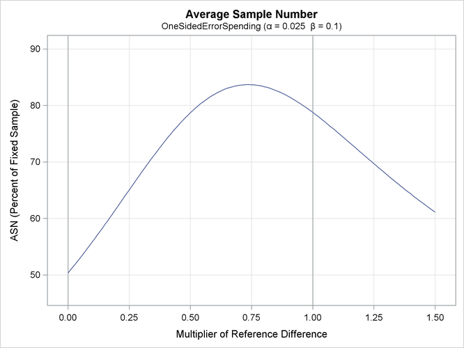
With the PLOTS=ASN option, the procedure displays a plot of expected sample sizes under various hypothetical references, as
shown in Output 89.8.5. By default, expected sample sizes under the hypotheses ![]() ,
, ![]() , are displayed, where
, are displayed, where ![]() is the alternative reference.
is the alternative reference.
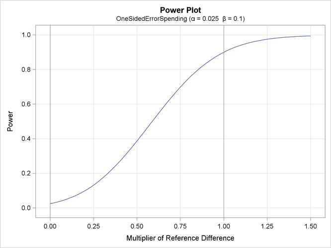
With the PLOTS=POWER option, the procedure displays a plot of the power curves under various hypothetical references for all
designs simultaneously, as shown in Output 89.8.6. By default, the option CREF= ![]() and powers under hypothetical references
and powers under hypothetical references ![]() are displayed, where
are displayed, where ![]() are values specified in the CREF= option. These CREF= values are displayed on the horizontal axis.
are values specified in the CREF= option. These CREF= values are displayed on the horizontal axis.
Under the null hypothesis, ![]() , the power is 0.025, the upper Type I error probability. Under the alternative hypothesis,
, the power is 0.025, the upper Type I error probability. Under the alternative hypothesis, ![]() , the power is 0.9, one minus the Type II error probability. The plot shows only minor difference between the two designs.
, the power is 0.9, one minus the Type II error probability. The plot shows only minor difference between the two designs.
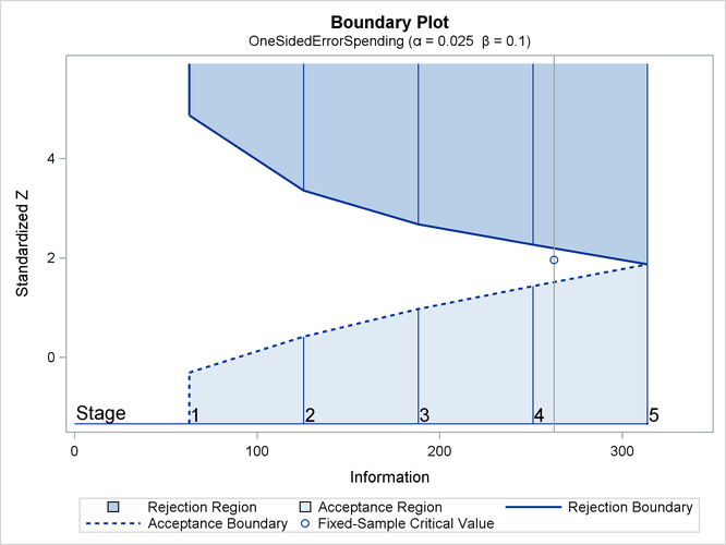
The "Boundary Information" table in Output 89.8.7 displays information level, alternative reference, and boundary values. By default (or equivalently if you specify BOUNDARYSCALE=STDZ),
the alternative reference and boundary values are displayed with the standardized Z scale. That is, the resulting standardized alternative reference at stage k is given by ![]() , where
, where ![]() is the specified alternative reference and
is the specified alternative reference and ![]() is the information level at stage k,
is the information level at stage k, ![]() .
.
Output 89.8.7: Boundary Information
| Boundary Information (Standardized Z Scale) Null Reference = 0 |
|||||
|---|---|---|---|---|---|
| _Stage_ | Alternative | Boundary Values | |||
| Information Level | Reference | Upper | |||
| Proportion | Actual | Upper | Beta | Alpha | |
| 1 | 0.2000 | 62.74393 | 1.58422 | -0.30338 | 4.87688 |
| 2 | 0.4000 | 125.4879 | 2.24043 | 0.41667 | 3.35706 |
| 3 | 0.6000 | 188.2318 | 2.74395 | 0.97165 | 2.67766 |
| 4 | 0.8000 | 250.9757 | 3.16844 | 1.43627 | 2.26535 |
| 5 | 1.0000 | 313.7196 | 3.54243 | 1.87522 | 1.87522 |
With ODS Graphics enabled, a detailed boundary plot with the rejection and acceptance regions is displayed, as shown in Output 89.8.8. This plot displays the boundary values in the "Boundary Information" table in Output 89.8.7.
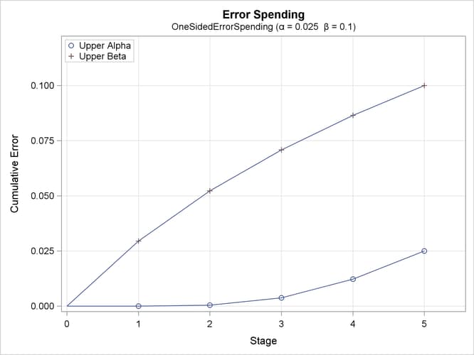
The "Error Spending Information" table in Output 89.8.9 displays cumulative error spending at each stage for each boundary.
With the PLOTS=ERRSPEND option, the procedure displays a plot of error spending for each boundary, as shown in Output 89.8.10. This plot displays the cumulative error spending at each stage in the "Error Spending Information" table in Output 89.8.9. The O’Brien-Fleming-type ![]() spending function is conservative in early stages because it uses much less at early stages than in the later stages. In
contrast, the Pocock-type
spending function is conservative in early stages because it uses much less at early stages than in the later stages. In
contrast, the Pocock-type ![]() spending function uses more at early stages than in the later stages.
spending function uses more at early stages than in the later stages.