The VARIOGRAM Procedure

You can choose between two approaches to select a theoretical semivariogram model and fit the empirical semivariance. The first one is manual fitting, in which a theoretical semivariogram model is selected based on visual inspection of the empirical semivariogram. For example, see Hohn (1988, p. 25) and comments from defendants of this approach in Olea (1999, p. 82). The second approach is to perform model fitting in an automated manner. For this task you can use methods such as least squares, maximum likelihood, and robust methods (Cressie, 1993, section 2.6).
The VARIOGRAM procedure features automated semivariogram model fitting that uses the weighted least squares (WLS) or the ordinary least squares (OLS) method. Use the MODEL statement to request that specific model forms or an array of candidate models be tested for optimal fitting to the empirical semivariance.
Assume that you compute first the empirical semivariance ![]() at MAXLAGS=k distance classes, where
at MAXLAGS=k distance classes, where ![]() can be either the classical estimate
can be either the classical estimate ![]() or the robust estimate
or the robust estimate ![]() , as shown in the section Theoretical and Computational Details of the Semivariogram. In fitting based on least squares, you want to estimate the parameters vector
, as shown in the section Theoretical and Computational Details of the Semivariogram. In fitting based on least squares, you want to estimate the parameters vector ![]() of the theoretical semivariance
of the theoretical semivariance ![]() that minimizes the sum of square differences
that minimizes the sum of square differences ![]() given by the expression
given by the expression
For ![]() , the weights are
, the weights are ![]() in the case of WLS and
in the case of WLS and ![]() in the case of OLS. Therefore, the parameters
in the case of OLS. Therefore, the parameters ![]() are estimated in OLS by minimizing
are estimated in OLS by minimizing
For WLS, Cressie (1985) investigated approximations for the variance of both the classical and robust empirical semivariances. Then, under the assumptions
of normally distributed observations and uncorrelated squared differences in the empirical semivariance, the approximate weighted
least squares estimate of the parameters ![]() can be obtained by minimizing
can be obtained by minimizing
where ![]() is the number of pairs of points in the ith distance lag.
is the number of pairs of points in the ith distance lag.
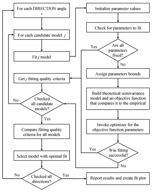
PROC VARIOGRAM relies on nonlinear optimization to minimize the least squares objective function ![]() . The outcome is the model that best fits the empirical semivariogram according to your criteria. The fitting process flow
is displayed in Figure 106.25. Goovaerts (1997, section 4.2.4) suggests that fitting a theoretical model should aim to capture the major spatial features. An accurate fit
is desirable, but overfitting does not offer advantages, because you might find yourself trying to model possibly spurious
details of the empirical semivariogram. At the same time, it is important to describe the correlation behavior accurately
near the semivariogram origin. As pointed out by Chilès and Delfiner (1999, pp. 104–105), a poor description of spatial continuity at small lags can lead to loss of optimality in kriging predictions
and erroneous reproduction of the variability in conditional simulations.
. The outcome is the model that best fits the empirical semivariogram according to your criteria. The fitting process flow
is displayed in Figure 106.25. Goovaerts (1997, section 4.2.4) suggests that fitting a theoretical model should aim to capture the major spatial features. An accurate fit
is desirable, but overfitting does not offer advantages, because you might find yourself trying to model possibly spurious
details of the empirical semivariogram. At the same time, it is important to describe the correlation behavior accurately
near the semivariogram origin. As pointed out by Chilès and Delfiner (1999, pp. 104–105), a poor description of spatial continuity at small lags can lead to loss of optimality in kriging predictions
and erroneous reproduction of the variability in conditional simulations.
The significance of achieving better accuracy near the semivariogram origin is an advantage of the WLS method compared to
OLS. In particular, the semivariance variance decreases when you get closer the origin ![]() , as suggested in the section Theoretical and Computational Details of the Semivariogram. The WLS weights are expressed as the inverse of this variance; as a result, WLS fitting is more accurate for distances
, as suggested in the section Theoretical and Computational Details of the Semivariogram. The WLS weights are expressed as the inverse of this variance; as a result, WLS fitting is more accurate for distances ![]() near the semivariogram origin. In contrast, the OLS approach performs a least squares overall best fit because it assumes
constant variance at all distances
near the semivariogram origin. In contrast, the OLS approach performs a least squares overall best fit because it assumes
constant variance at all distances ![]() . Another advantage of WLS over OLS is that OLS falsely assumes that the differences in the optimization process are normally
distributed and independent. However, WLS has the disadvantage that the weights depend on the fitting parameters.
. Another advantage of WLS over OLS is that OLS falsely assumes that the differences in the optimization process are normally
distributed and independent. However, WLS has the disadvantage that the weights depend on the fitting parameters.
Depending on your application, you can use WLS or OLS with PROC VARIOGRAM to fit classical semivariance. Other fitting methods include maximum likelihood approaches that rely crucially on the normality assumption for the data distribution, and the generalized least squares method that offers better accuracy but is computationally more demanding. You can find extensive discussions about these issues in Cressie (1993, section 2.3), Jian, Olea, and Yu (1996), Stein (1988), and Schabenberger and Gotway (2005).
The sections Parameter Initialization and Quality of Fit provide details and insight about semivariogram fitting, in addition to ways to cope with poor fits or no fit at all. These strategies can help you reach a meaningful description of spatial correlation in your problem.