The QUANTSELECT Procedure

This simulation study exemplifies the unity of motive and effect for the PROC QUANTSELECT procedure. The following statements generate a data set that is based on a naive instrumental model (Chernozhukov and Hansen, 2008):
%let seed=321;
%let p=20;
%let n=3000;

data analysisData;
   array x{&p} x1-x&p;
   do i=1 to &n;
      U  = ranuni(&seed);
      x1 = ranuni(&seed);
      x2 = ranexp(&seed);
      x3 = abs(rannor(&seed));
      y  = x1*(U-0.1) + x2*(U*U-0.25) + x3*(exp(U)-exp(0.9));
      do j=4 to &p;
         x{j} = ranuni(&seed);
      end;
      output;
   end;
run;
Variable U of the data set indicates the true quantile level of the response y conditional on ![]() .
.
Let ![]() denote the underlying quantile regression model, where
denote the underlying quantile regression model, where ![]() . Then, the true parameter functions are
. Then, the true parameter functions are
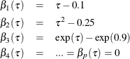
It is easy to see that, at ![]() , only
, only ![]() and
and ![]() are nonzero parameters. Therefore, an effective effect selection method should select
are nonzero parameters. Therefore, an effective effect selection method should select ![]() and
and ![]() and drop all the other effects in this data set at
and drop all the other effects in this data set at ![]() . By the same rationale,
. By the same rationale, ![]() and
and ![]() should be selected at
should be selected at ![]() with
with ![]() and
and ![]() , and
, and ![]() and
and ![]() should be selected at
should be selected at ![]() with
with ![]() and
and ![]() .
.
The following statements use PROC QUANTSELECT with the adaptive LASSO method:
proc quantselect data=analysisData;
   model y= x1-x&p / quantile=0.1 0.5 0.9
         selection=lasso(adaptive);
   output out=out p=pred;
run;
Output 82.1.1 shows that, by default, the CHOOSE= and STOP= options are both set to SBC.
Output 82.1.1: Model Information
| Model Information | |
|---|---|
| Data Set | WORK.ANALYSISDATA |
| Dependent Variable | y |
| Selection Method | Adaptive LASSO |
| Quantile Type | Single Level |
| Stop Criterion | SBC |
| Choose Criterion | SBC |
The selected effects and the relevant estimates are shown in Output 82.1.2 for ![]() , Output 82.1.3 for
, Output 82.1.3 for ![]() , and Output 82.1.4 for
, and Output 82.1.4 for ![]() . You can see that the adaptive LASSO method correctly selects active effects for all three quantile levels.
. You can see that the adaptive LASSO method correctly selects active effects for all three quantile levels.
Output 82.1.2: Parameter Estimates at ![]()
| Selected Effects: | Intercept x2 x3 |
|---|
| Parameter Estimates | |||
|---|---|---|---|
| Parameter | DF | Estimate | Standardized Estimate |
| Intercept | 1 | 0.011793 | 0 |
| x2 | 1 | -0.228709 | -0.218287 |
| x3 | 1 | -1.379907 | -0.784520 |
Output 82.1.3: Parameter Estimates at ![]()
| Selected Effects: | Intercept x1 x3 |
|---|
| Parameter Estimates | |||
|---|---|---|---|
| Parameter | DF | Estimate | Standardized Estimate |
| Intercept | 1 | 0.011778 | 0 |
| x1 | 1 | 0.425843 | 0.118792 |
| x3 | 1 | -0.863316 | -0.490822 |
Output 82.1.4: Parameter Estimates at ![]()
| Selected Effects: | Intercept x1 x2 |
|---|
| Parameter Estimates | |||
|---|---|---|---|
| Parameter | DF | Estimate | Standardized Estimate |
| Intercept | 1 | -0.007738 | 0 |
| x1 | 1 | 0.782942 | 0.218407 |
| x2 | 1 | 0.576445 | 0.550177 |
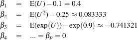
The QUANTSELECT procedure can perform effect selection not only at a single quantile level but also for the entire quantile
process. You can specify the QUANTILE=PROCESS option to do effect selection for the entire quantile process. With the QUANTILE=PROCESS
option specified, the ParameterEstimates table produced by the QUANTSELECT procedure actually shows the mean prediction model
of y conditional on ![]() . In this simulation study, the true mean model is
. In this simulation study, the true mean model is
where
The following statements perform effect selection for the quantile process with the forward selection method.
proc quantselect data=analysisData;
   model y= x1-x&p / quantile=process(ntau=all)
         selection=forward;
run;
Output 82.1.5 shows that, by default, the SELECT= and STOP= options are both set to SBC. The selected effects and the relevant estimates for the conditional mean model are shown in Output 82.1.6.
Output 82.1.5: Model Information
| Model Information | |
|---|---|
| Data Set | WORK.ANALYSISDATA |
| Dependent Variable | y |
| Selection Method | Forward |
| Quantile Type | Process |
| Select Criterion | SBC |
| Stop Criterion | SBC |
| Choose Criterion | SBC |
Output 82.1.6: Parameter Estimates
| Parameter Estimates | |||
|---|---|---|---|
| Parameter | DF | Estimate | Standardized Estimate |
| Intercept | 1 | 0.007833 | 0 |
| x1 | 1 | 0.418825 | 0.116834 |
| x2 | 1 | 0.094791 | 0.090472 |
| x3 | 1 | -0.785686 | -0.446687 |
Linear regression is the most popular method for estimating conditional means. The following statements show how to select effects with the GLMSELECT procedure, and Output 82.1.7 shows the resulting selected effects and their estimates. You can see that the mean estimates from the QUANTSELECT procedure are similar to those from the GLMSELECT procedure. However, quantile regression can provide detailed distribution information, which is not available from linear regression.
proc glmselect data=analysisData;
   model y= x1-x3 / selection=forward(select=sbc stop=sbc choose=sbc);
run;
Output 82.1.7: Parameter Estimates
| Parameter Estimates | ||||
|---|---|---|---|---|
| Parameter | DF | Estimate | Standard Error | t Value |
| Intercept | 1 | -0.010143 | 0.043129 | -0.24 |
| x1 | 1 | 0.434553 | 0.057385 | 7.57 |
| x2 | 1 | 0.114183 | 0.016771 | 6.81 |
| x3 | 1 | -0.797194 | 0.028156 | -28.31 |