The PRINQUAL Procedure
- Overview
- Getting Started
-
Syntax

-
DetailsThe Three Methods of Variable TransformationUnderstanding How PROC PRINQUAL WorksSplinesMissing ValuesControlling the Number of IterationsPerforming a Principal Component Analysis of Transformed DataUsing the MAC MethodOutput Data SetAvoiding Constant TransformationsConstant VariablesCharacter OPSCORE VariablesREITERATE Option UsagePassive ObservationsComputational ResourcesDisplayed OutputODS Table NamesODS Graphics
-
Examples
- References
In the following example, PROC PRINQUAL uses the MTV method to linearize a curved scatter plot. Let
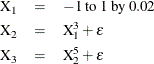
where ![]() is normal error.
is normal error.
These three variables define a curved swarm of points in three-dimensional space. First, the SGSCATTER procedure is used to display two-dimensional views of these data. Next, PROC PRINQUAL is used to straighten the scatter plot, making it more one-dimensional by finding a smooth transformation of each variable. The N=1 option in the PROC PRINQUAL statement requests one principal component. The TRANSFORM statement requests a cubic spline transformation with nine knots. Splines are curves, which are usually required to be continuous and smooth. See the section Splines for more information about splines. See Smith (1979) for an excellent introduction to splines.
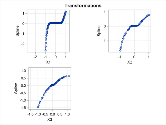
PROC PRINQUAL transforms each variable to be as much as possible like the first principal component (or more generally, to be close to the space defined by the first N= principal components). One component accounts for 92 percent of the variance of the untransformed data and over 99 percent of the variance of the transformed data (see Figure 78.5). Note that the results did not converge in the default 50 iterations, so more iterations were requested using the MAXITER= option. The transformations are requested by specifying PLOTS=TRANSFORMATION and are displayed in Figure 78.6.
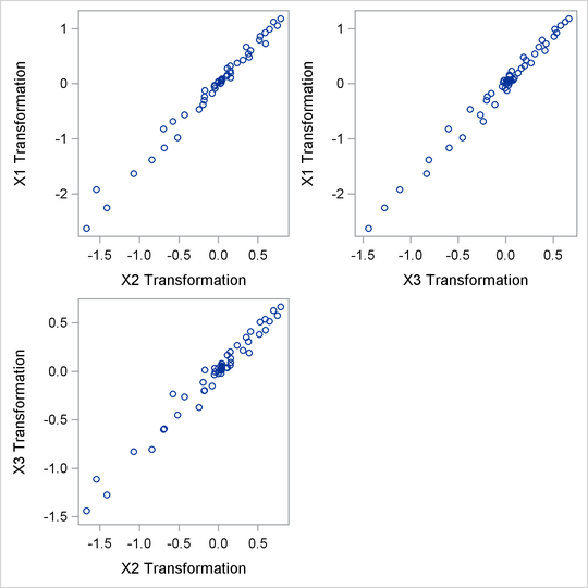
PROC PRINQUAL creates an output data set that contains both the original and transformed variables. The original variables
are named X1, X2, and X3, and the transformed variables are named TX1, TX2, and TX3. The transformed variables are displayed using the SGSCATTER procedure in Figure 78.7.
The following statements produce Figure 78.4 through Figure 78.7:
ods graphics on;

* Generate Three-Dimensional Data;
data X;
   do X1 = -1 to 1 by 0.02;
      X2 = X1 ** 3 + 0.05 * normal(7);
      X3 = X1 ** 5 + 0.05 * normal(7);
      output;
   end;
run;

proc sgscatter data=x;
   plot x1*x2 x1*x3 x3*x2;
run;

* Try to Straighten the Scatter Plot;
proc prinqual data=X n=1 maxiter=2000 plots=transformation out=results;
   title 'Linearize the Scatter Plot';
   transform spline(X1-X3 / nknots=9);
run;


* Plot the Linearized Scatter Plot;
proc sgscatter data=results;
   plot tx1*tx2 tx1*tx3 tx3*tx2;
run;
The three-dimensional data in Figure 78.4 and Figure 78.7 are displayed in three two-dimensional plots, arrayed as if they were three faces of a cube that was flattened as you might flatten a box.

Figure 78.5: PRINQUAL Iteration History
| Linearize the Scatter Plot |
| The PRINQUAL Procedure |
| PRINQUAL MTV Algorithm Iteration History |
| Iteration Number |
Average Change |
Maximum Change |
Proportion of Variance |
Criterion Change |
Note |
|---|---|---|---|---|---|
| 1 | 0.15125 | 0.93453 | 0.92376 | ||
| 2 | 0.04589 | 0.14682 | 0.98030 | 0.05653 | |
| 3 | 0.03154 | 0.10125 | 0.98626 | 0.00596 | |
| 4 | 0.02258 | 0.06890 | 0.98890 | 0.00265 | |
| 5 | 0.01682 | 0.04777 | 0.99028 | 0.00137 | |
| 6 | 0.01297 | 0.03782 | 0.99106 | 0.00078 | |
| 7 | 0.01032 | 0.03029 | 0.99154 | 0.00048 | |
| . | |||||
| . | |||||
| . | |||||
| 1670 | 0.00001 | 0.00005 | 0.99371 | 0.00000 | |
| 1671 | 0.00001 | 0.00005 | 0.99371 | 0.00000 | |
| 1672 | 0.00001 | 0.00005 | 0.99371 | 0.00000 | Converged |
Algorithm converged. |