The PLS Procedure

This example demonstrates issues in spectrometric calibration. The data (Umetrics 1995) consist of spectrographic readings on 33 samples containing known concentrations of two amino acids, tyrosine and tryptophan.
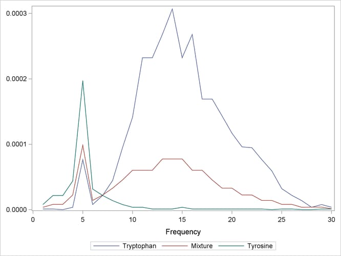
The spectra are measured at 30 frequencies across the overall range of frequencies. For example, Output 74.3.1 shows the observed spectra for three samples, one with only tryptophan, one with only tyrosine, and one with a mixture of
the two, all at a total concentration of ![]() .
.
Of the 33 samples, 18 are used as a training set and 15 as a test set. The data originally appear in McAvoy et al. (1989).
These data were created in a lab, with the concentrations fixed in order to provide a wide range of applicability for the
model. You want to use a linear function of the logarithms of the spectra to predict the logarithms of tyrosine and tryptophan
concentration, as well as the logarithm of the total concentration. Actually, because of the possibility of zeros in both
the responses and the predictors, slightly different transformations are used. The following statements create SAS data sets
containing the training and test data, named ftrain and ftest, respectively.
data ftrain;
   input obsnam $ tot tyr f1-f30 @@;
   try = tot - tyr;
   if (tyr) then tyr_log = log10(tyr); else tyr_log = -8;
   if (try) then try_log = log10(try); else try_log = -8;
   tot_log = log10(tot);
   datalines;
17mix35 0.00003 0
 -6.215 -5.809 -5.114 -3.963 -2.897 -2.269 -1.675 -1.235
 -0.900 -0.659 -0.497 -0.395 -0.335 -0.315 -0.333 -0.377
 -0.453 -0.549 -0.658 -0.797 -0.878 -0.954 -1.060 -1.266
 -1.520 -1.804 -2.044 -2.269 -2.496 -2.714
19mix35 0.00003 3E-7
 -5.516 -5.294 -4.823 -3.858 -2.827 -2.249 -1.683 -1.218
 -0.907 -0.658 -0.501 -0.400 -0.345 -0.323 -0.342 -0.387
 -0.461 -0.554 -0.665 -0.803 -0.887 -0.960 -1.072 -1.272
 -1.541 -1.814 -2.058 -2.289 -2.496 -2.712
21mix35 0.00003 7.5E-7
 -5.519 -5.294 -4.501 -3.863 -2.827 -2.280 -1.716 -1.262
 -0.939 -0.694 -0.536 -0.444 -0.384 -0.369 -0.377 -0.421
 -0.495 -0.596 -0.706 -0.824 -0.917 -0.988 -1.103 -1.294
 -1.565 -1.841 -2.084 -2.320 -2.521 -2.729
23mix35 0.00003 1.5E-6

   ... more lines ...

mix6    0.0001 0.00009
 -1.140 -0.757 -0.497 -0.362 -0.329 -0.412 -0.513 -0.647
 -0.772 -0.877 -0.958 -1.040 -1.104 -1.162 -1.233 -1.317
 -1.425 -1.543 -1.661 -1.804 -1.877 -1.959 -2.034 -2.249
 -2.502 -2.732 -2.964 -3.142 -3.313 -3.576
;
data ftest;
   input obsnam $ tot tyr f1-f30 @@;
   try = tot - tyr;
   if (tyr) then tyr_log = log10(tyr); else tyr_log = -8;
   if (try) then try_log = log10(try); else try_log = -8;
   tot_log = log10(tot);
   datalines;
43trp6  1E-6 0
 -5.915 -5.918 -6.908 -5.428 -4.117 -5.103 -4.660 -4.351
 -4.023 -3.849 -3.634 -3.634 -3.572 -3.513 -3.634 -3.572
 -3.772 -3.772 -3.844 -3.932 -4.017 -4.023 -4.117 -4.227
 -4.492 -4.660 -4.855 -5.428 -5.103 -5.428
59mix6  1E-6 1E-7
 -5.903 -5.903 -5.903 -5.082 -4.213 -5.083 -4.838 -4.639
 -4.474 -4.213 -4.001 -4.098 -4.001 -4.001 -3.907 -4.001
 -4.098 -4.098 -4.206 -4.098 -4.213 -4.213 -4.335 -4.474
 -4.639 -4.838 -4.837 -5.085 -5.410 -5.410
51mix6  1E-6 2.5E-7
 -5.907 -5.907 -5.415 -4.843 -4.213 -4.843 -4.843 -4.483
 -4.343 -4.006 -4.006 -3.912 -3.830 -3.830 -3.755 -3.912
 -4.006 -4.001 -4.213 -4.213 -4.335 -4.483 -4.483 -4.642
 -4.841 -5.088 -5.088 -5.415 -5.415 -5.415
49mix6  1E-6 5E-7

   ... more lines ...

tyro2   0.0001 0.0001
 -1.081 -0.710 -0.470 -0.337 -0.327 -0.433 -0.602 -0.841
 -1.119 -1.423 -1.750 -2.121 -2.449 -2.818 -3.110 -3.467
 -3.781 -4.029 -4.241 -4.366 -4.501 -4.366 -4.501 -4.501
 -4.668 -4.668 -4.865 -4.865 -5.109 -5.111
;
The following statements fit a PLS model with 10 factors.
proc pls data=ftrain nfac=10;
   model tot_log tyr_log try_log = f1-f30;
run;
The table shown in Output 74.3.2 indicates that only three or four factors are required to explain almost all of the variation in both the predictors and the responses.
Output 74.3.2: Amount of Training Set Variation Explained
| Percent Variation Accounted for by Partial Least Squares Factors |
||||
|---|---|---|---|---|
| Number of Extracted Factors |
Model Effects | Dependent Variables | ||
| Current | Total | Current | Total | |
| 1 | 81.1654 | 81.1654 | 48.3385 | 48.3385 |
| 2 | 16.8113 | 97.9768 | 32.5465 | 80.8851 |
| 3 | 1.7639 | 99.7407 | 11.4438 | 92.3289 |
| 4 | 0.1951 | 99.9357 | 3.8363 | 96.1652 |
| 5 | 0.0276 | 99.9634 | 1.6880 | 97.8532 |
| 6 | 0.0132 | 99.9765 | 0.7247 | 98.5779 |
| 7 | 0.0052 | 99.9817 | 0.2926 | 98.8705 |
| 8 | 0.0053 | 99.9870 | 0.1252 | 98.9956 |
| 9 | 0.0049 | 99.9918 | 0.1067 | 99.1023 |
| 10 | 0.0034 | 99.9952 | 0.1684 | 99.2707 |
In order to choose the optimal number of PLS factors, you can explore how well models based on the training data with different
numbers of factors fit the test data. To do so, use the CV=TESTSET option, with an argument pointing to the test data set ftest. The following statements also employ the ODS Graphics features in PROC PLS to display the cross validation results in a
plot.
ods graphics on;

proc pls data=ftrain nfac=10 cv=testset(ftest)
                             cvtest(stat=press seed=12345);
   model tot_log tyr_log try_log = f1-f30;
run;
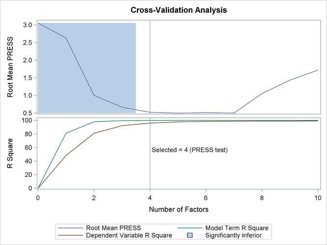
The tabular results of the test set validation are shown in Output 74.3.3, and the graphical results are shown in Output 74.3.4. They indicate that, although five PLS factors give the minimum predicted residual sum of squares, the residuals for four factors are insignificantly different from those for five. Thus, the smaller model is preferred.
Output 74.3.3: Test Set Validation for the Number of PLS Factors
| Test Set Validation for the Number of Extracted Factors |
||
|---|---|---|
| Number of Extracted Factors |
Root Mean PRESS | Prob > PRESS |
| 0 | 3.056797 | <.0001 |
| 1 | 2.630561 | <.0001 |
| 2 | 1.00706 | 0.0070 |
| 3 | 0.664603 | 0.0020 |
| 4 | 0.521578 | 0.3800 |
| 5 | 0.500034 | 1.0000 |
| 6 | 0.513561 | 0.5100 |
| 7 | 0.501431 | 0.6870 |
| 8 | 1.055791 | 0.1530 |
| 9 | 1.435085 | 0.1010 |
| 10 | 1.720389 | 0.0320 |
| Minimum root mean PRESS | 0.5000 |
|---|---|
| Minimizing number of factors | 5 |
| Smallest number of factors with p > 0.1 | 4 |
| Percent Variation Accounted for by Partial Least Squares Factors |
||||
|---|---|---|---|---|
| Number of Extracted Factors |
Model Effects | Dependent Variables | ||
| Current | Total | Current | Total | |
| 1 | 81.1654 | 81.1654 | 48.3385 | 48.3385 |
| 2 | 16.8113 | 97.9768 | 32.5465 | 80.8851 |
| 3 | 1.7639 | 99.7407 | 11.4438 | 92.3289 |
| 4 | 0.1951 | 99.9357 | 3.8363 | 96.1652 |
The factor loadings show how the PLS factors are constructed from the centered and scaled predictors. For spectral calibration, it is useful to plot the loadings against the frequency. In many cases, the physical meanings that can be attached to factor loadings help to validate the scientific interpretation of the PLS model. You can use ODS Graphics with PROC PLS to plot the loadings for the four PLS factors against frequency, as shown in the following statements.
proc pls data=ftrain nfac=4 plot=XLoadingProfiles;
   model tot_log tyr_log try_log = f1-f30;
run;

ods graphics off;
The resulting plot is shown in Output 74.3.5.
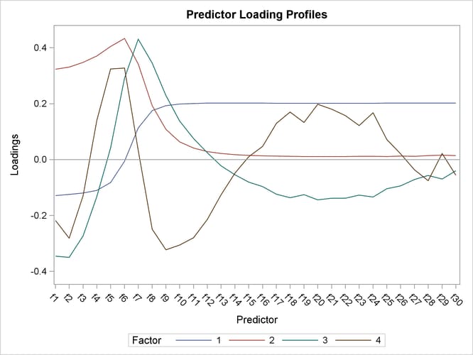
Notice that all four factors handle frequencies below and above about 7 or 8 differently. For example, the first factor is very nearly a simple contrast between the averages of the two sets of frequencies, and the second factor appears to be approximately a weighted sum of only the frequencies in the first set.