The NLMIXED Procedure
-
Overview

-
Getting Started
-
Syntax
-
DetailsModeling Assumptions and NotationIntegral ApproximationsBuilt-in Log-Likelihood FunctionsOptimization AlgorithmsFinite-Difference Approximations of DerivativesHessian ScalingActive Set MethodsLine-Search MethodsRestricting the Step LengthComputational ProblemsCovariance MatrixPredictionComputational ResourcesDisplayed OutputODS Table Names
-
Examples
- References
A popular application of nonlinear mixed models is in the field of pharmacokinetics, which studies how a drug disperses through a living individual. This example considers the theophylline data from Pinheiro and Bates (1995). Serum concentrations of the drug theophylline are measured in 12 subjects over a 25-hour period after oral administration. The data are as follows.
data theoph;
   input subject time conc dose wt;
   datalines;
 1  0.00  0.74 4.02 79.6
 1  0.25  2.84 4.02 79.6
 1  0.57  6.57 4.02 79.6
 1  1.12 10.50 4.02 79.6
 1  2.02  9.66 4.02 79.6
 1  3.82  8.58 4.02 79.6
 1  5.10  8.36 4.02 79.6
 1  7.03  7.47 4.02 79.6

   ... more lines ...

12 24.15  1.17 5.30 60.5
;
Pinheiro and Bates (1995) consider the following first-order compartment model for these data:
where ![]() is the observed concentration of the ith subject at time t, D is the dose of theophylline,
is the observed concentration of the ith subject at time t, D is the dose of theophylline, ![]() is the elimination rate constant for subject i,
is the elimination rate constant for subject i, ![]() is the absorption rate constant for subject i,
is the absorption rate constant for subject i, ![]() is the clearance for subject i, and
is the clearance for subject i, and ![]() are normal errors. To allow for random variability between subjects, they assume
are normal errors. To allow for random variability between subjects, they assume
where the ![]() s denote fixed-effects parameters and the
s denote fixed-effects parameters and the ![]() s denote random-effects parameters with an unknown covariance matrix.
s denote random-effects parameters with an unknown covariance matrix.
The PROC NLMIXED statements to fit this model are as follows:
proc nlmixed data=theoph;
parms beta1=-3.22 beta2=0.47 beta3=-2.45
s2b1 =0.03 cb12 =0 s2b2 =0.4 s2=0.5;
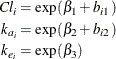
cl = exp(beta1 + b1);
ka = exp(beta2 + b2);
ke = exp(beta3);
pred = dose*ke*ka*(exp(-ke*time)-exp(-ka*time))/cl/(ka-ke);
model conc ~ normal(pred,s2);
random b1 b2 ~ normal([0,0],[s2b1,cb12,s2b2]) subject=subject;
run;
The PARMS statement specifies starting values for the three ![]() s and four variance-covariance parameters. The clearance and rate constants are defined using SAS programming statements,
and the conditional model for the data is defined to be normal with mean
s and four variance-covariance parameters. The clearance and rate constants are defined using SAS programming statements,
and the conditional model for the data is defined to be normal with mean pred and variance s2. The two random effects are b1 and b2, and their joint distribution is defined in the RANDOM statement. Brackets are used in defining their mean vector (two zeros) and the lower triangle of their variance-covariance
matrix (a general ![]() matrix). The SUBJECT= variable is
matrix). The SUBJECT= variable is subject.
The results from this analysis are as follows.
Output 68.1.1: Model Specification for One-Compartment Model
| Specifications | |
|---|---|
| Data Set | WORK.THEOPH |
| Dependent Variable | conc |
| Distribution for Dependent Variable | Normal |
| Random Effects | b1 b2 |
| Distribution for Random Effects | Normal |
| Subject Variable | subject |
| Optimization Technique | Dual Quasi-Newton |
| Integration Method | Adaptive Gaussian Quadrature |
The “Specifications” table lists the setup of the model (Output 68.1.1). The “Dimensions” table indicates that there are 132 observations, 12 subjects, and 7 parameters. PROC NLMIXED selects 5 quadrature points for each random effect, producing a total grid of 25 points over which quadrature is performed (Output 68.1.2).
Output 68.1.2: Dimensions Table for One-Compartment Model
| Dimensions | |
|---|---|
| Observations Used | 132 |
| Observations Not Used | 0 |
| Total Observations | 132 |
| Subjects | 12 |
| Max Obs per Subject | 11 |
| Parameters | 7 |
| Quadrature Points | 5 |
The “Parameters” table lists the 7 parameters, their starting values, and the initial evaluation of the negative log likelihood using adaptive Gaussian quadrature (Output 68.1.3). The “Iteration History” table indicates that 10 steps are required for the dual quasi-Newton algorithm to achieve convergence.
Output 68.1.3: Starting Values and Iteration History
| Parameters | |||||||
|---|---|---|---|---|---|---|---|
| beta1 | beta2 | beta3 | s2b1 | cb12 | s2b2 | s2 | NegLogLike |
| -3.22 | 0.47 | -2.45 | 0.03 | 0 | 0.4 | 0.5 | 177.789945 |
| Iteration History | ||||||
|---|---|---|---|---|---|---|
| Iter | Calls | NegLogLike | Diff | MaxGrad | Slope | |
| 1 | 7 | 177.776248 | 0.013697 | 2.873367 | -63.0744 | |
| 2 | 11 | 177.7643 | 0.011948 | 1.698144 | -4.75239 | |
| 3 | 14 | 177.757264 | 0.007036 | 1.297439 | -1.97311 | |
| 4 | 17 | 177.755688 | 0.001576 | 1.441408 | -0.49772 | |
| 5 | 20 | 177.7467 | 0.008988 | 1.132279 | -0.8223 | |
| 6 | 24 | 177.746401 | 0.000299 | 0.831293 | -0.00244 | |
| 7 | 27 | 177.746318 | 0.000083 | 0.724198 | -0.00789 | |
| 8 | 31 | 177.74574 | 0.000578 | 0.180018 | -0.00583 | |
| 9 | 34 | 177.745736 | 3.88E-6 | 0.017958 | -8.25E-6 | |
| 10 | 37 | 177.745736 | 3.222E-8 | 0.000143 | -6.51E-8 | |
| NOTE: GCONV convergence criterion satisfied. |
Output 68.1.4: Fit Statistics for One-Compartment Model
| Fit Statistics | |
|---|---|
| -2 Log Likelihood | 355.5 |
| AIC (smaller is better) | 369.5 |
| AICC (smaller is better) | 370.4 |
| BIC (smaller is better) | 372.9 |
The “Fit Statistics” table lists the final optimized values of the log-likelihood function and information criteria in the “smaller is better” form (Output 68.1.4).
The “Parameter Estimates” table contains the maximum likelihood estimates of the parameters (Output 68.1.5). Both s2b1 and s2b2 are marginally significant, indicating between-subject variability in the clearances and absorption rate constants, respectively.
There does not appear to be a significant covariance between them, as seen by the estimate of cb12.
Output 68.1.5: Parameter Estimates for One-Compartment Model
| Parameter Estimates | |||||||||
|---|---|---|---|---|---|---|---|---|---|
| Parameter | Estimate | Standard Error | DF | t Value | Pr > |t| | Alpha | Lower | Upper | Gradient |
| beta1 | -3.2268 | 0.05950 | 10 | -54.23 | <.0001 | 0.05 | -3.3594 | -3.0942 | -0.00009 |
| beta2 | 0.4806 | 0.1989 | 10 | 2.42 | 0.0363 | 0.05 | 0.03745 | 0.9238 | 3.645E-7 |
| beta3 | -2.4592 | 0.05126 | 10 | -47.97 | <.0001 | 0.05 | -2.5734 | -2.3449 | 0.000039 |
| s2b1 | 0.02803 | 0.01221 | 10 | 2.30 | 0.0446 | 0.05 | 0.000828 | 0.05524 | -0.00014 |
| cb12 | -0.00127 | 0.03404 | 10 | -0.04 | 0.9710 | 0.05 | -0.07712 | 0.07458 | -0.00007 |
| s2b2 | 0.4331 | 0.2005 | 10 | 2.16 | 0.0561 | 0.05 | -0.01354 | 0.8798 | -6.98E-6 |
| s2 | 0.5016 | 0.06837 | 10 | 7.34 | <.0001 | 0.05 | 0.3493 | 0.6540 | 6.133E-6 |
The estimates of ![]() ,
, ![]() , and
, and ![]() are close to the adaptive quadrature estimates listed in Table 3 of Pinheiro and Bates (1995). However, Pinheiro and Bates use a Cholesky-root parameterization for the random-effects variance matrix and a logarithmic
parameterization for the residual variance. The PROC NLMIXED statements using their parameterization are as follows, and results
are similar.
are close to the adaptive quadrature estimates listed in Table 3 of Pinheiro and Bates (1995). However, Pinheiro and Bates use a Cholesky-root parameterization for the random-effects variance matrix and a logarithmic
parameterization for the residual variance. The PROC NLMIXED statements using their parameterization are as follows, and results
are similar.
proc nlmixed data=theoph;
   parms ll1=-1.5 l2=0 ll3=-0.1 beta1=-3 beta2=0.5 beta3=-2.5 ls2=-0.7;
   s2   = exp(ls2);
   l1   = exp(ll1);
   l3   = exp(ll3);
   s2b1 = l1*l1*s2;
   cb12 = l2*l1*s2;
   s2b2 = (l2*l2 + l3*l3)*s2;
   cl   = exp(beta1 + b1);
   ka   = exp(beta2 + b2);
   ke   = exp(beta3);
   pred = dose*ke*ka*(exp(-ke*time)-exp(-ka*time))/cl/(ka-ke);
   model conc   ~ normal(pred,s2);
   random b1 b2 ~ normal([0,0],[s2b1,cb12,s2b2]) subject=subject;
run;