The MCMC Procedure
-
Overview

-
Getting Started
-
Syntax
-
DetailsHow PROC MCMC WorksBlocking of ParametersSampling MethodsTuning the Proposal DistributionDirect SamplingConjugate SamplingInitial Values of the Markov ChainsAssignments of ParametersStandard DistributionsUsage of Multivariate DistributionsSpecifying a New DistributionUsing Density Functions in the Programming StatementsTruncation and CensoringSome Useful SAS FunctionsMatrix Functions in PROC MCMCCreate Design MatrixModeling Joint LikelihoodRegenerating Diagnostics PlotsCaterpillar PlotAutocall Macros for PostprocessingGamma and Inverse-Gamma DistributionsPosterior Predictive DistributionHandling of Missing DataFunctions of Random-Effects ParametersFloating Point Errors and OverflowsHandling Error MessagesComputational ResourcesDisplayed OutputODS Table NamesODS Graphics
-
ExamplesSimulating Samples From a Known DensityBox-Cox TransformationLogistic Regression Model with a Diffuse PriorLogistic Regression Model with Jeffreys’ PriorPoisson RegressionNonlinear Poisson Regression ModelsLogistic Regression Random-Effects ModelNonlinear Poisson Regression Multilevel Random-Effects ModelMultivariate Normal Random-Effects ModelMissing at Random AnalysisNonignorably Missing Data (MNAR) AnalysisChange Point ModelsExponential and Weibull Survival AnalysisTime Independent Cox ModelTime Dependent Cox ModelPiecewise Exponential Frailty ModelNormal Regression with Interval CensoringConstrained AnalysisImplement a New Sampling AlgorithmUsing a Transformation to Improve MixingGelman-Rubin Diagnostics
- References
This example illustrates how to fit a piecewise exponential frailty model using PROC MCMC. Part of the notation and presentation in this example follows Clayton (1991) and the Luek example in Spiegelhalter et al. (1996a).
Generally speaking, the proportional hazards model assumes the hazard function,
where ![]() indexes subject,
indexes subject, ![]() is the baseline hazard function, and
is the baseline hazard function, and ![]() are the covariates for subject i. If you define
are the covariates for subject i. If you define ![]() to be the number of observed failures of the ith subject up to time t, then the hazard function for the ith subject can be seen as a special case of a multiplicative intensity model (Clayton, 1991). The intensity process for
to be the number of observed failures of the ith subject up to time t, then the hazard function for the ith subject can be seen as a special case of a multiplicative intensity model (Clayton, 1991). The intensity process for ![]() becomes
becomes
where ![]() indicates observation of the subject at time t (taking the value of 1 if the subject is observed and 0 otherwise). Under noninformative censoring, the corresponding likelihood is proportional to
indicates observation of the subject at time t (taking the value of 1 if the subject is observed and 0 otherwise). Under noninformative censoring, the corresponding likelihood is proportional to
where ![]() is the increment of
is the increment of ![]() over the small time interval
over the small time interval ![]() : it takes a value of 1 if the subject i fails in the time interval, 0 otherwise. This is a Poisson kernel with the random variable being the increments of
: it takes a value of 1 if the subject i fails in the time interval, 0 otherwise. This is a Poisson kernel with the random variable being the increments of ![]() and the means
and the means ![]()
where
and
The integral is the increment in the integrated baseline hazard function that occurs during the time interval ![]() .
.
This formulation provides an alternative way to fit a piecewise exponential model. You partition the time axis to a few intervals,
where each interval has its own hazard rate, ![]() . You count the
. You count the ![]() and
and ![]() in each interval, and fit a Poisson model to each count.
in each interval, and fit a Poisson model to each count.
The following DATA step creates the data set Blind (Lin, 1994) that represents 197 diabetic patients who have a high risk of experiencing blindness in both eyes as defined by DRS criteria:
title 'Piecewise Exponential Model';
data Blind;
   input ID Time Status DiabeticType Treatment @@;
   datalines;
   5 46.23 0 1 1    5 46.23 0 1 0   14 42.50 0 0 1   14 31.30 1 0 0
  16 42.27 0 0 1   16 42.27 0 0 0   25 20.60 0 0 1   25 20.60 0 0 0
  29 38.77 0 0 1   29  0.30 1 0 0   46 65.23 0 0 1   46 54.27 1 0 0
  49 63.50 0 0 1   49 10.80 1 0 0   56 23.17 0 0 1   56 23.17 0 0 0

   ... more lines ...

1705  8.00 0 0 1 1705  8.00 0 0 0 1717 51.60 0 1 1 1717 42.33 1 1 0
1727 49.97 0 1 1 1727  2.90 1 1 0 1746 45.90 0 0 1 1746  1.43 1 0 0
1749 41.93 0 1 1 1749 41.93 0 1 0
;
One eye of each patient is treated with laser photocoagulation. The hypothesis of interest is whether the laser treatment
delays the occurrence of blindness. The following variables are included in Blind:
-
ID, patient’s identification -
Time, failure time -
Status, event indicator (0=censored and 1=uncensored) -
Treatment, treatment received (1=laser photocoagulation and 0=otherwise) -
DiabeticType, type of diabetes (0=juvenile onset with age of onset at 20 or under, and 1= adult onset with age of onset over 20)
For illustrational purposes, a piecewise exponential model that ignores the patient-level frailties is first fit to the entire data set. The formulation of the Poisson counting process makes it straightforward to add the frailty terms, as it is demonstrated later.
The following statements create a partition (of length 8) along the time axis, with ![]() , with
, with ![]() and
and ![]() for all i. The time intervals are stored in the
for all i. The time intervals are stored in the Partition data set:
data partition;
   input int_1-int_9;
   datalines;
   0.1  6.545  13.95  26.47  38.8  45.88  54.35  62 80
;
To obtain reasonable estimates, placing an equal number of observations in each interval is recommended. You can find the
partition points by calculating the percentile statistics of the time variable (for example, by using the UNIVARIATE procedure).
The following regression model and prior distributions are used in the analysis:
The following statements calculate ![]() for each observation i, at every time point t in the
for each observation i, at every time point t in the Partition data set. The statements also find the observed failure time interval, ![]() , for each observation:
, for each observation:
%let n = 8;
data _a;
   set blind;
   if _n_ eq 1 then set partition;
   array int[*] int_:;
   array Y[&n];
   array dN[&n];
   do k = 1 to (dim(int)-1);
      Y[k] = (time - int[k] + 0.001 >= 0);
      dN[k] = Y[k] * ( int[k+1] - time - 0.001 >= 0) * status;
   end;
   output;
   drop int_: k;
run;
The DATA step reads in the Blind data set. At the first observation, it also reads in the Partition data set. The first ARRAY statement creates the int array and name the elements int_:. Because the names match the variable names in the Partition data set, all values of the int_: variables (there is only one observation) in the Partition data set are therefore stored in the int array. The next two ARRAY statements create arrays Y and dN, each with length 8. They store values of ![]() and
and ![]() , resulting from each failure time in the
, resulting from each failure time in the Blind data set.
The following statements print the first 10 observations of the constructed data set _a and display them in Output 59.16.1:
proc print data=_a(obs=10);
run;
Output 59.16.1: First 10 Observations of the Data Set _a
| Piecewise Exponential Model |
| Obs | ID | Time | Status | DiabeticType | Treatment | Y1 | Y2 | Y3 | Y4 | Y5 | Y6 | Y7 | Y8 | dN1 | dN2 | dN3 | dN4 | dN5 | dN6 | dN7 | dN8 |
|---|---|---|---|---|---|---|---|---|---|---|---|---|---|---|---|---|---|---|---|---|---|
| 1 | 5 | 46.23 | 0 | 1 | 1 | 1 | 1 | 1 | 1 | 1 | 1 | 0 | 0 | 0 | 0 | 0 | 0 | 0 | 0 | 0 | 0 |
| 2 | 5 | 46.23 | 0 | 1 | 0 | 1 | 1 | 1 | 1 | 1 | 1 | 0 | 0 | 0 | 0 | 0 | 0 | 0 | 0 | 0 | 0 |
| 3 | 14 | 42.50 | 0 | 0 | 1 | 1 | 1 | 1 | 1 | 1 | 0 | 0 | 0 | 0 | 0 | 0 | 0 | 0 | 0 | 0 | 0 |
| 4 | 14 | 31.30 | 1 | 0 | 0 | 1 | 1 | 1 | 1 | 0 | 0 | 0 | 0 | 0 | 0 | 0 | 1 | 0 | 0 | 0 | 0 |
| 5 | 16 | 42.27 | 0 | 0 | 1 | 1 | 1 | 1 | 1 | 1 | 0 | 0 | 0 | 0 | 0 | 0 | 0 | 0 | 0 | 0 | 0 |
| 6 | 16 | 42.27 | 0 | 0 | 0 | 1 | 1 | 1 | 1 | 1 | 0 | 0 | 0 | 0 | 0 | 0 | 0 | 0 | 0 | 0 | 0 |
| 7 | 25 | 20.60 | 0 | 0 | 1 | 1 | 1 | 1 | 0 | 0 | 0 | 0 | 0 | 0 | 0 | 0 | 0 | 0 | 0 | 0 | 0 |
| 8 | 25 | 20.60 | 0 | 0 | 0 | 1 | 1 | 1 | 0 | 0 | 0 | 0 | 0 | 0 | 0 | 0 | 0 | 0 | 0 | 0 | 0 |
| 9 | 29 | 38.77 | 0 | 0 | 1 | 1 | 1 | 1 | 1 | 0 | 0 | 0 | 0 | 0 | 0 | 0 | 0 | 0 | 0 | 0 | 0 |
| 10 | 29 | 0.30 | 1 | 0 | 0 | 1 | 0 | 0 | 0 | 0 | 0 | 0 | 0 | 1 | 0 | 0 | 0 | 0 | 0 | 0 | 0 |
The first subject in _a experienced blindness in the left eye at time 46.23, and the time falls in the sixth interval as defined in the Partition data set. Therefore, Y1 through Y6 all take a value of 1, and Y7 and Y8 are 0. The variable dN# takes on a value of 1 if the subject is observed to go blind in that interval. Since the first observation is censored (status == 1), the actual failure time is unknown. Hence all dN# are 0. The first observed failure time occurs in observation number 4 (the right eye of the second subject), where the time variable takes a value of 31.30, Y1 through Y4 are 1, and dN4 is 1.
Note that each observation in the _a data set has 8 Y and 8 dN, meaning that you would need eight MODEL statements in a PROC MCMC call, each for a Poisson likelihood. Alternatively, you can expand _a, put one Y and one dN in every observation, and fit the data using a single MODEL statement in PROC MCMC. The following statements expand the data set _a and save the results in the data set _b:
data _b;
   set _a;
   array y[*] y:;
   array dn[*] dn:;
   do i = 1 to (dim(y));
      y_val       = y[i];
      dn_val      = dn[i];
      int_index   = i;
      output;
   end;
   keep y_: dn_: diabetictype treatment int_index id;
run;

data _b;
   set _b;
   rename y_val=Y dn_val=dN;
run;
You can use the following PROC PRINT statements to see the first few observations in _b:
proc print data=_b(obs=10);
run;
Output 59.16.2: First 20 Observations of the Data Set _b
| Obs | ID | DiabeticType | Treatment | Y | dN | int_index |
|---|---|---|---|---|---|---|
| 1 | 5 | 1 | 1 | 1 | 0 | 1 |
| 2 | 5 | 1 | 1 | 1 | 0 | 2 |
| 3 | 5 | 1 | 1 | 1 | 0 | 3 |
| 4 | 5 | 1 | 1 | 1 | 0 | 4 |
| 5 | 5 | 1 | 1 | 1 | 0 | 5 |
| 6 | 5 | 1 | 1 | 1 | 0 | 6 |
| 7 | 5 | 1 | 1 | 0 | 0 | 7 |
| 8 | 5 | 1 | 1 | 0 | 0 | 8 |
| 9 | 5 | 1 | 0 | 1 | 0 | 1 |
| 10 | 5 | 1 | 0 | 1 | 0 | 2 |
The data set _b now contains 3,152 observations (see Output 59.16.2 for the first few observations). The Time and Status variables are no longer needed; hence they are discarded from the data set. The int_index variable is an index variable that indicates interval membership of each observation.
Because the variable Y does not contribute to the likelihood calculation when it takes a value of 0 (it amounts to a Poisson likelihood that has
a mean and response variable that are both 0), you can remove these observations. This speeds up the calculation in PROC MCMC:
data inputdata;
   set _b;
   if Y > 0;
run;
The data set Inputdata has 1,775 observations, as opposed to 3,152 observations in _b. The following statements fit a piecewise exponential model in PROC MCMC:
proc mcmc data=inputdata nmc=10000 outpost=postout seed=12351
maxtune=5;
ods select PostSumInt ESS;
parms beta1-beta3 0;
prior beta: ~ normal(0, var = 1e6);
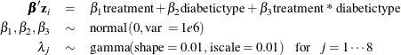
random lambda ~ gamma(0.01, iscale = 0.01) subject=int_index;
bZ = beta1*treatment + beta2*diabetictype + beta3*treatment*diabetictype;
idt = exp(bz) * lambda;
model dN ~ poisson(idt);
run;
The PARMS statement declares three regression parameters, beta1–beta3. The PRIOR statement specifies a noninformative normal prior on the regression coefficients. The RANDOM statement specifies the random effect, lambda, its prior distribution, and interval membership which is indexed by the data set variable int_index.
The symbol bZ calculates the regression mean, and the symbol idt is the mean of the Poisson likelihood. It corresponds to the equation
Note that the ![]() term is omitted in the assignment statement because
term is omitted in the assignment statement because Y takes only the value of 1 in the input data set.
Output 59.16.3 displays posterior estimates of the three regression parameters.
Output 59.16.3: Posterior Summary Statistics
| Posterior Summaries and Intervals | |||||
|---|---|---|---|---|---|
| Parameter | N | Mean | Standard Deviation |
95% HPD Interval | |
| beta1 | 10000 | -0.4174 | 0.2129 | -0.8121 | 0.0203 |
| beta2 | 10000 | 0.3138 | 0.1956 | -0.0885 | 0.6958 |
| beta3 | 10000 | -0.7899 | 0.3308 | -1.4300 | -0.1046 |
To understand the results, you can create a ![]() table (Table 59.49) and plug in the posterior mean estimates to the regression model. A –0.41 estimate for subjects who received laser treatment
and had juvenile diabetes suggests that the laser treatment is effective in delaying blindness. And the effect is much more
pronounced (–0.80) for adult subjects who have diabetes and received treatment.
table (Table 59.49) and plug in the posterior mean estimates to the regression model. A –0.41 estimate for subjects who received laser treatment
and had juvenile diabetes suggests that the laser treatment is effective in delaying blindness. And the effect is much more
pronounced (–0.80) for adult subjects who have diabetes and received treatment.
Table 59.49: Estimates of Regression Effects in the Survival Model
|
|
Diabetic Type |
||
|
0 |
1 |
||
|
Treatment |
0 |
0 |
0.32 |
|
1 |
–0.41 |
–0.80 |
|
You can also use the macro %CATER (Caterpillar Plot) to draw a caterpillar plot to visualize the eight hazards in the model:
ods graphics on;
%cater(data=postout, var=lambda_:);
ods graphics off;
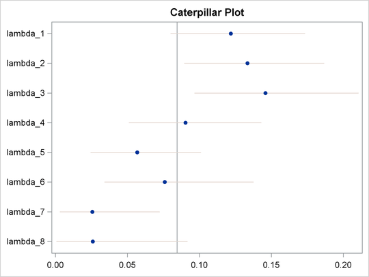
The fitted hazards show a nonconstant underlying hazard function (read along the y-axis as lambda_# are hazards along the time-axis) in the model.
Now suppose you want to include patient-level information and fit a frailty model to the blind data set, where the random effect enters the model through the regression term, where the subject is indexed by the variable
ID in the data.
where id indexes patient.
The actual coding in PROC MCMC of a piecewise exponential frailty model is rather straightforward:
ods select none;
proc mcmc data=inputdata nmc=10000 outpost=postout seed=12351
stats=summary diag=none;
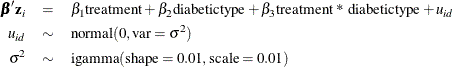
parms beta1-beta3 0 s2;
prior beta: ~ normal(0, var = 1e6);
prior s2 ~ igamma(0.01, scale=0.01);
random lambda ~ gamma(0.01, iscale = 0.01) subject=int_index;
random u ~ normal(0, var=s2) subject=id;
bZ = beta1*treatment + beta2*diabetictype + beta3*treatment*diabetictype + u;
idt = exp(bZ) * lambda;
model dN ~ poisson(idt);
run;
A second RANDOM statement defines a subject-level random effect u, and the random-effects parameters enter the model in the term for the regression mean, bZ. An additional model parameter, s2, the variance of the random-effects parameters, is needed for the model. The results are not shown here.