The LOGISTIC Procedure
- Overview
- Getting Started
-
Syntax
 PROC LOGISTIC StatementBY StatementCLASS StatementCODE StatementCONTRAST StatementEFFECT StatementEFFECTPLOT StatementESTIMATE StatementEXACT StatementEXACTOPTIONS StatementFREQ StatementID StatementLSMEANS StatementLSMESTIMATE StatementMODEL StatementNLOPTIONS StatementODDSRATIO StatementOUTPUT StatementROC StatementROCCONTRAST StatementSCORE StatementSLICE StatementSTORE StatementSTRATA StatementTEST StatementUNITS StatementWEIGHT Statement
 -
DetailsMissing ValuesResponse Level OrderingLink Functions and the Corresponding DistributionsDetermining Observations for Likelihood ContributionsIterative Algorithms for Model FittingConvergence CriteriaExistence of Maximum Likelihood EstimatesEffect-Selection MethodsModel Fitting InformationGeneralized Coefficient of DeterminationScore Statistics and TestsConfidence Intervals for ParametersOdds Ratio EstimationRank Correlation of Observed Responses and Predicted ProbabilitiesLinear Predictor, Predicted Probability, and Confidence LimitsClassification TableOverdispersionThe Hosmer-Lemeshow Goodness-of-Fit TestReceiver Operating Characteristic CurvesTesting Linear Hypotheses about the Regression CoefficientsRegression DiagnosticsScoring Data SetsConditional Logistic RegressionExact Conditional Logistic RegressionInput and Output Data SetsComputational ResourcesDisplayed OutputODS Table NamesODS Graphics
-
ExamplesStepwise Logistic Regression and Predicted ValuesLogistic Modeling with Categorical PredictorsOrdinal Logistic RegressionNominal Response Data: Generalized Logits ModelStratified SamplingLogistic Regression DiagnosticsROC Curve, Customized Odds Ratios, Goodness-of-Fit Statistics, R-Square, and Confidence LimitsComparing Receiver Operating Characteristic CurvesGoodness-of-Fit Tests and SubpopulationsOverdispersionConditional Logistic Regression for Matched Pairs DataFirth’s Penalized Likelihood Compared with Other ApproachesComplementary Log-Log Model for Infection RatesComplementary Log-Log Model for Interval-Censored Survival TimesScoring Data SetsUsing the LSMEANS StatementPartial Proportional Odds Model
- References
The method of maximum likelihood described in the preceding sections relies on large-sample asymptotic normality for the validity
of estimates and especially of their standard errors. When you do not have a large sample size compared to the number of parameters,
this approach might be inappropriate and might result in biased inferences. This situation typically arises when your data
are stratified and you fit intercepts to each stratum so that the number of parameters is of the same order as the sample
size. For example, in a ![]() matched pairs study with n pairs and p covariates, you would estimate
matched pairs study with n pairs and p covariates, you would estimate ![]() intercept parameters and p slope parameters. Taking the stratification into account by “conditioning out” (and not estimating) the stratum-specific intercepts gives consistent and asymptotically normal MLEs for the slope coefficients.
See Breslow and Day (1980) and Stokes, Davis, and Koch (2012) for more information. If your nuisance parameters are not just stratum-specific intercepts, you can perform an exact conditional logistic regression.
intercept parameters and p slope parameters. Taking the stratification into account by “conditioning out” (and not estimating) the stratum-specific intercepts gives consistent and asymptotically normal MLEs for the slope coefficients.
See Breslow and Day (1980) and Stokes, Davis, and Koch (2012) for more information. If your nuisance parameters are not just stratum-specific intercepts, you can perform an exact conditional logistic regression.
For each stratum h, ![]() , number the observations as
, number the observations as ![]() so that hi indexes the ith observation in stratum h. Denote the p covariates for the hith observation as
so that hi indexes the ith observation in stratum h. Denote the p covariates for the hith observation as ![]() and its binary response as
and its binary response as ![]() , and let
, and let ![]() ,
, ![]() , and
, and ![]() . Let the dummy variables
. Let the dummy variables ![]() , be indicator functions for the strata (
, be indicator functions for the strata (![]() if the observation is in stratum h), and denote
if the observation is in stratum h), and denote ![]() for the hith observation,
for the hith observation, ![]() , and
, and ![]() . Denote
. Denote ![]() ) and
) and ![]() . Arrange the observations in each stratum h so that
. Arrange the observations in each stratum h so that ![]() for
for ![]() , and
, and ![]() for
for ![]() . Suppose all observations have unit frequency.
. Suppose all observations have unit frequency.
Consider the binary logistic regression model written as
where the parameter vector ![]() consists of
consists of ![]() ,
, ![]() is the intercept for stratum
is the intercept for stratum ![]() , and
, and ![]() is the parameter vector for the p covariates.
is the parameter vector for the p covariates.
From the section Determining Observations for Likelihood Contributions, you can write the likelihood contribution of observation ![]() as
as
where ![]() when the response takes Ordered Value 1, and
when the response takes Ordered Value 1, and ![]() otherwise.
otherwise.
The full likelihood is
![\[ L(\btheta ) = \prod _{h=1}^{H} \prod _{i=1}^{n_ h} L_{hi}(\btheta ) = \frac{e^{\mb {y}{\bX ^{^*}}\btheta }}{\prod _{h=1}^{H} \prod _{i=1}^{n_ h} \left(1+e^{{\mb {x}^*_{hi}}\btheta }\right)} \]](images/statug_logistic0609.png)
Unconditional likelihood inference is based on maximizing this likelihood function.
When your nuisance parameters are the stratum-specific intercepts ![]() , and the slopes
, and the slopes ![]() are your parameters of interest, “conditioning out” the nuisance parameters produces the conditional likelihood (Lachin, 2000)
are your parameters of interest, “conditioning out” the nuisance parameters produces the conditional likelihood (Lachin, 2000)
where the summation is over all ![]() subsets
subsets ![]() of
of ![]() observations chosen from the
observations chosen from the ![]() observations in stratum h. Note that the nuisance parameters have been factored out of this equation.
observations in stratum h. Note that the nuisance parameters have been factored out of this equation.
For conditional asymptotic inference, maximum likelihood estimates ![]() of the regression parameters are obtained by maximizing the conditional likelihood, and asymptotic results are applied to
the conditional likelihood function and the maximum likelihood estimators. A relatively fast method of computing this conditional
likelihood and its derivatives is given by Gail, Lubin, and Rubinstein (1981) and Howard (1972). The optimization techniques can be controlled by specifying the NLOPTIONS statement.
of the regression parameters are obtained by maximizing the conditional likelihood, and asymptotic results are applied to
the conditional likelihood function and the maximum likelihood estimators. A relatively fast method of computing this conditional
likelihood and its derivatives is given by Gail, Lubin, and Rubinstein (1981) and Howard (1972). The optimization techniques can be controlled by specifying the NLOPTIONS statement.
Sometimes the log likelihood converges but the estimates diverge. This condition is flagged by having inordinately large standard errors for some of your parameter estimates, and can be monitored by specifying the ITPRINT option. Unfortunately, broad existence criteria such as those discussed in the section Existence of Maximum Likelihood Estimates do not exist for this model. It might be possible to circumvent such a problem by standardizing your independent variables before fitting the model.
Diagnostics are used to indicate observations that might have undue influence on the model fit or that might be outliers. Further investigation should be performed before removing such an observation from the data set.
The derivations in this section use an augmentation method described by Storer and Crowley (1985), which provides an estimate of the “one-step” DFBETAS estimates advocated by Pregibon (1984). The method also provides estimates of conditional stratum-specific predicted values, residuals, and leverage for each observation. The augmentation method can take a lot of time and memory.
Following Storer and Crowley (1985), the log-likelihood contribution can be written as
![\begin{eqnarray*} l_ h & =& \log (L_ h) = \mb {y}_ h’\bgamma _ h - a(\bgamma _ h)\quad \mbox{where} \\ a(\bgamma _ h) & =& \log \left[\sum \prod _{j=j_1}^{j_{m_ h}}\exp (\bgamma _{hj})\right] \end{eqnarray*}](images/statug_logistic0616.png)
and the h subscript on matrices indicates the submatrix for the stratum, ![]() , and
, and ![]() . Then the gradient and information matrix are
. Then the gradient and information matrix are
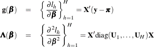
where
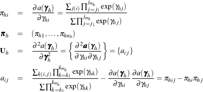
and where ![]() is the conditional stratum-specific probability that subject i in stratum h is a case, the summation on
is the conditional stratum-specific probability that subject i in stratum h is a case, the summation on ![]() is over all subsets from
is over all subsets from ![]() of size
of size ![]() that contain the index i, and the summation on
that contain the index i, and the summation on ![]() is over all subsets from
is over all subsets from ![]() of size
of size ![]() that contain the indices i and j.
that contain the indices i and j.
To produce the true one-step estimate ![]() , start at the MLE
, start at the MLE ![]() , delete the hith observation, and use this reduced data set to compute the next Newton-Raphson step. Note that if there is only one event
or one nonevent in a stratum, deletion of that single observation is equivalent to deletion of the entire stratum. The augmentation
method does not take this into account.
, delete the hith observation, and use this reduced data set to compute the next Newton-Raphson step. Note that if there is only one event
or one nonevent in a stratum, deletion of that single observation is equivalent to deletion of the entire stratum. The augmentation
method does not take this into account.
The augmented model is
where ![]() has a 1 in the hith coordinate, and use
has a 1 in the hith coordinate, and use ![]() as the initial estimate for
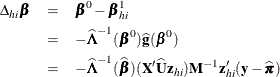
as the initial estimate for ![]() . The gradient and information matrix before the step are
. The gradient and information matrix before the step are
 = \left[\begin{array}{c}{\bm {0}}\\ {y_{hi}-{\pi }_{hi}}\end{array}\right]\\ \bLambda (\bbeta ^0) & =& \left[\begin{array}{c}{\bX ’}\\ {\mb {z}_{hi}’}\end{array}\right]{\bU }\left[{\bX }\quad {\mb {z}_{hi}}\right] = \left[\begin{array}{cc}\bLambda ({\bbeta }) & \bX ’{\bU }\mb {z}_{hi}\\ \mb {z}_{hi}’{\bU }\bX & \mb {z}_{hi}’{\bU }\mb {z}_{hi} \end{array}\right] \end{eqnarray*}](images/statug_logistic0629.png)
Inserting the ![]() and
and ![]() into the Gail, Lubin, and Rubinstein (1981) algorithm provides the appropriate estimates of
into the Gail, Lubin, and Rubinstein (1981) algorithm provides the appropriate estimates of ![]() and
and ![]() . Indicate these estimates with
. Indicate these estimates with ![]() ,
, ![]() ,
, ![]() , and
, and ![]() .
.
DFBETA is computed from the information matrix as
where
For each observation in the data set, a DFBETA statistic is computed for each parameter ![]() ,
, ![]() , and standardized by the standard error of
, and standardized by the standard error of ![]() from the full data set to produce the estimate of DFBETAS.
from the full data set to produce the estimate of DFBETAS.
The estimated leverage is defined as
This definition of leverage produces different values from those defined by Pregibon (1984); Moolgavkar, Lustbader, and Venzon (1985); Hosmer and Lemeshow (2000); however, it has the advantage that no extra computations beyond those for the DFBETAS are required.
The estimated residuals ![]() are obtained from
are obtained from ![]() , and the weights, or predicted probabilities, are then
, and the weights, or predicted probabilities, are then ![]() . The residuals are standardized and reported as (estimated) Pearson residuals:
. The residuals are standardized and reported as (estimated) Pearson residuals:
where ![]() is the number of events in the observation and
is the number of events in the observation and ![]() is the number of trials.
is the number of trials.
The STDRES option in the INFLUENCE option computes the standardized Pearson residual:
For events/trials MODEL statement syntax, treat each observation as two observations (the first for the nonevents and the
second for the events) with frequencies ![]() and
and ![]() , and augment the model with a matrix
, and augment the model with a matrix ![]() instead of a single
instead of a single ![]() vector. Writing
vector. Writing ![]() in the preceding section results in the following gradient and information matrix:
in the preceding section results in the following gradient and information matrix:
![\begin{eqnarray*} \mb {g}(\bbeta ^0) & =& \left[\begin{array}{c}{\bm {0}}\\ {f_{h,2i-1}(y_{h,2i-1}-{\pi }_{h,2i-1})}\\ {f_{h,2i}(y_{h,2i}-{\pi }_{h,2i})}\\ \end{array}\right]\\ \bLambda (\bbeta ^0) & =& \left[\begin{array}{cc}\bLambda ({\bbeta }) & \bX ’\mbox{diag}(\mb {f}){\bU }\mbox{diag}(\mb {f})\bZ _{hi}\\ \bZ _{hi}’\mbox{diag}(\mb {f}){\bU }\mbox{diag}(\mb {f})\bX & \bZ _{hi}’\mbox{diag}(\mb {f}){\bU }\mbox{diag}(\mb {f})\bZ _{hi} \end{array}\right] \end{eqnarray*}](images/statug_logistic0654.png)
The predicted probabilities are then ![]() , while the leverage and the DFBETAS are produced from
, while the leverage and the DFBETAS are produced from ![]() in a fashion similar to that for the preceding single-trial equations.
in a fashion similar to that for the preceding single-trial equations.