Example 49.2 Controlling the Plotting of Survival Estimates

Recall the breast cancer data in the example in the section Getting Started: ICLIFETEST Procedure. The following statements compute complementary log-log transformed pointwise confidence limits for the two treatment groups and plot them:

proc iclifetest data=BCS plots=survival(cl) impute(seed=1234);
   strata trt;
   time (lTime, rTime);
run;

The two areas overlap a lot before the 20th month. After that, the radiation-only group tends to have higher survival rate than the radiation-plus-chemotherapy group. That is, patients who receive only radiation tend to survive longer to experience cosmetic deterioration than those who receive both treatments.

Output 49.2.1: Nonparametric Survival Estimates for Breast Cancer Data

The dashed lines visually connect the survival estimates across Turnbull intervals for which the estimates are not defined. You can choose not to display the dashed lines by specifying the NODASH option as follows:

proc iclifetest data=BCS plots=survival(cl nodash) impute(seed=1234);
   strata trt;
   time (lTime, rTime);
run;

In Output 49.2.2, the survival estimates are plotted only for the time intervals for which estimates can be obtained.

Output 49.2.2: Nonparametric Survival Estimates

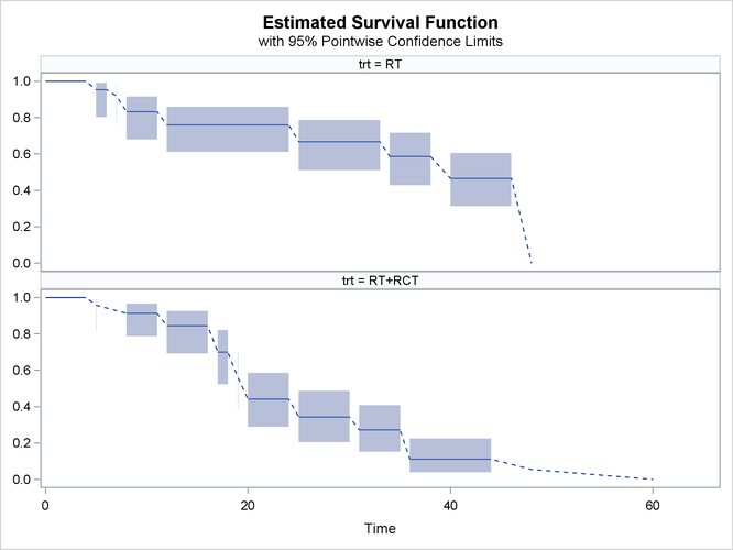
If the overlaid plot becomes too busy, then it might be necessary to plot the survival estimates separately. You can request a paneled display of individual survival estimate by specifying the STRATA=PANEL option as follows:

proc iclifetest data=BCS plots=survival(cl strata=panel) impute(seed=1234);
   strata trt;
   time (lTime, rTime);
run;

Now the output survival estimates for different treatments are plotted in different panels, as shown in Output 49.2.3.

Output 49.2.3: Paneled Survival Plot

The ICLIFETEST Procedure

Example 49.2 Controlling the Plotting of Survival Estimates