The GLMSELECT Procedure
-
Overview

- Getting Started
-
Syntax
-
DetailsModel-Selection MethodsModel Selection IssuesCriteria Used in Model Selection MethodsCLASS Variable Parameterization and the SPLIT OptionMacro Variables Containing Selected ModelsUsing the STORE StatementBuilding the SSCP MatrixModel AveragingUsing Validation and Test DataCross ValidationExternal Cross ValidationDisplayed OutputODS Table NamesODS Graphics
-
Examples
- References
The Sashelp.Baseball data set contains salary and performance information for Major League Baseball players who played at least one game in both
the 1986 and 1987 seasons, excluding pitchers. The salaries (Sports Illustrated, April 20, 1987) are for the 1987 season and the performance measures are from 1986 (Collier Books, The 1987 Baseball Encyclopedia Update). The following step displays in Figure 47.1 the variables in the data set:
proc contents varnum data=sashelp.baseball;
   ods select position;
run;
Figure 47.1: Sashelp.Baseball Data Set
| Variables in Creation Order | ||||
|---|---|---|---|---|
| # | Variable | Type | Len | Label |
| 1 | Name | Char | 18 | Player's Name |
| 2 | Team | Char | 14 | Team at the End of 1986 |
| 3 | nAtBat | Num | 8 | Times at Bat in 1986 |
| 4 | nHits | Num | 8 | Hits in 1986 |
| 5 | nHome | Num | 8 | Home Runs in 1986 |
| 6 | nRuns | Num | 8 | Runs in 1986 |
| 7 | nRBI | Num | 8 | RBIs in 1986 |
| 8 | nBB | Num | 8 | Walks in 1986 |
| 9 | YrMajor | Num | 8 | Years in the Major Leagues |
| 10 | CrAtBat | Num | 8 | Career Times at Bat |
| 11 | CrHits | Num | 8 | Career Hits |
| 12 | CrHome | Num | 8 | Career Home Runs |
| 13 | CrRuns | Num | 8 | Career Runs |
| 14 | CrRbi | Num | 8 | Career RBIs |
| 15 | CrBB | Num | 8 | Career Walks |
| 16 | League | Char | 8 | League at the End of 1986 |
| 17 | Division | Char | 8 | Division at the End of 1986 |
| 18 | Position | Char | 8 | Position(s) in 1986 |
| 19 | nOuts | Num | 8 | Put Outs in 1986 |
| 20 | nAssts | Num | 8 | Assists in 1986 |
| 21 | nError | Num | 8 | Errors in 1986 |
| 22 | Salary | Num | 8 | 1987 Salary in $ Thousands |
| 23 | Div | Char | 16 | League and Division |
| 24 | logSalary | Num | 8 | Log Salary |
Suppose you want to investigate whether you can model the players’ salaries for the 1987 season based on performance measures for the previous season. The aim is to obtain a parsimonious model that does not overfit this particular data, making it useful for prediction. This example shows how you can use PROC GLMSELECT as a starting point for such an analysis. Since the variation of salaries is much greater for the higher salaries, it is appropriate to apply a log transformation to the salaries before doing the model selection.
The following code selects a model with the default settings:
ods graphics on;
proc glmselect data=sashelp.baseball plots=all;
   class league division;
   model logSalary = nAtBat nHits nHome nRuns nRBI nBB
                     yrMajor crAtBat crHits crHome crRuns crRbi
                     crBB league division nOuts nAssts nError
                   / details=all stats=all;
run;
ods graphics off;
PROC GLMSELECT performs effect selection where effects can contain classification variables that you specify in a CLASS statement. The “Class Level Information” table shown in Figure 47.2 lists the levels of the classification variables Division and League.
Figure 47.2: Class Level Information
| Class Level Information | ||
|---|---|---|
| Class | Levels | Values |
| League | 2 | American National |
| Division | 2 | East West |
When you specify effects that contain classification variables, the number of parameters is usually larger than the number of effects. The “Dimensions” table in Figure 47.3 shows the number of effects and the number of parameters considered.
Figure 47.4: Model Information
| Data Set | SASHELP.BASEBALL |
|---|---|
| Dependent Variable | logSalary |
| Selection Method | Stepwise |
| Select Criterion | SBC |
| Stop Criterion | SBC |
| Effect Hierarchy Enforced | None |
You find details of the default search settings in the “Model Information” table shown in Figure 47.4. The default selection method is a variant of the traditional stepwise selection where the decisions about what effects to add or drop at any step and when to terminate the selection are both based on the Schwarz Bayesian information criterion (SBC). The effect in the current model whose removal yields the maximal decrease in the SBC statistic is dropped provided this lowers the SBC value. Once no decrease in the SBC value can be obtained by dropping an effect in the model, the effect whose addition to the model yields the lowest SBC statistic is added and the whole process is repeated. The method terminates when dropping or adding any effect increases the SBC statistic.
Figure 47.5: Candidates for Entry at Step Two
| Best 10 Entry Candidates | ||
|---|---|---|
| Rank | Effect | SBC |
| 1 | nHits | -252.5794 |
| 2 | nAtBat | -241.5789 |
| 3 | nRuns | -240.1010 |
| 4 | nRBI | -232.2880 |
| 5 | nBB | -223.3741 |
| 6 | nHome | -208.0565 |
| 7 | nOuts | -205.8107 |
| 8 | Division | -194.4688 |
| 9 | CrBB | -191.5141 |
| 10 | nAssts | -190.9425 |
The DETAILS=ALL option requests details of each step of the selection process. The “Best 10 Entry Candidates” table at each step shows the candidates for inclusion or removal at that step ranked from best to worst in terms of the selection criterion, which in this example is the SBC statistic. By default only the 10 best candidates are shown. Figure 47.5 shows the candidate table at step two.
To help in the interpretation of the selection process, you can use graphics supported by PROC GLMSELECT. ODS Graphics must
be enabled before requesting plots. For general information about ODS Graphics, see Chapter 21: Statistical Graphics Using ODS. With ODS Graphics enabled, the PLOTS=ALL option together with the DETAILS=STEPS option in the MODEL statement produces a needle plot view of the “Candidates” tables. The plot corresponding to the “Candidates” table at step two is shown in Figure 47.6. You can see that adding the effect nHits yields the smallest SBC value, and so this effect is added at step two.

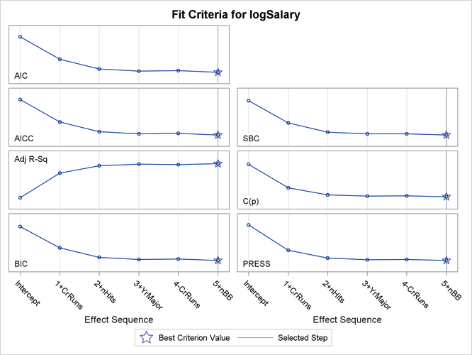
The “Stepwise Selection Summary” table in Figure 47.7 shows the effect that was added or dropped at each step of the selection process together with fit statistics for the model at each step. The STATS=ALL option in the MODEL statement requests that all the available fit statistics are displayed. See the section Criteria Used in Model Selection Methods for descriptions and formulas. The criterion panel in Figure 47.8 provides a graphical view of the progression of these fit criteria as the selection process evolves. Note that none of these criteria has a local optimum before step five.
Figure 47.7: Selection Summary Table
| Stepwise Selection Summary | |||||||||||||||
|---|---|---|---|---|---|---|---|---|---|---|---|---|---|---|---|
| Step | Effect Entered |
Effect Removed |
Number Effects In |
Number Parms In |
Model R-Square |
Adjusted R-Square |
AIC | AICC | BIC | CP | SBC | PRESS | ASE | F Value | Pr > F |
| 0 | Intercept | 1 | 1 | 0.0000 | 0.0000 | 204.2238 | 204.2699 | -60.6397 | 375.9275 | -57.2041 | 208.7381 | 0.7877 | 0.00 | 1.0000 | |
| 1 | CrRuns | 2 | 2 | 0.4187 | 0.4165 | 63.5391 | 63.6318 | -200.7872 | 111.2315 | -194.3166 | 123.9195 | 0.4578 | 188.01 | <.0001 | |
| 2 | nHits | 3 | 3 | 0.5440 | 0.5405 | 1.7041 | 1.8592 | -261.8807 | 33.4438 | -252.5794 | 97.6368 | 0.3592 | 71.42 | <.0001 | |
| 3 | YrMajor | 4 | 4 | 0.5705 | 0.5655 | -12.0208 | -11.7873 | -275.3333 | 18.5870 | -262.7322 | 92.2998 | 0.3383 | 15.96 | <.0001 | |
| 4 | CrRuns | 3 | 3 | 0.5614 | 0.5581 | -8.5517 | -8.3967 | -271.9095 | 22.3357 | -262.8353 | 93.1482 | 0.3454 | 5.44 | 0.0204 | |
| 5 | nBB | 4 | 4 | 0.5818 | 0.5770* | -19.0690* | -18.8356* | -282.1700* | 11.3524* | -269.7804* | 89.5434* | 0.3294 | 12.62 | 0.0005 | |
| * Optimal Value Of Criterion | |||||||||||||||
The stop reason and stop details tables in Figure 47.9 gives details of why the selection process terminated. This table shows that at step five the best add candidate, Division, and the best drop candidate, nBB, yield models with SBC values of –268.6094 and –262.8353, respectively. Both of these values are larger than the current
SBC value of –269.7804, and so the selection process stops at the model at step five.
Figure 47.9: Stopping Details
| Selection stopped at a local minimum of the SBC criterion. |
| Stop Details | ||||
|---|---|---|---|---|
| Candidate For |
Effect | Candidate SBC |
Compare SBC |
|
| Entry | Division | -268.6094 | > | -269.7804 |
| Removal | nBB | -262.8353 | > | -269.7804 |
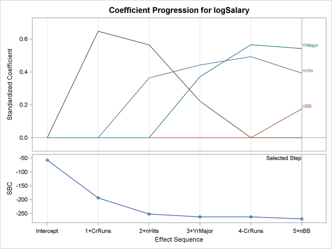
The coefficient panel in Figure 47.10 enables you to visualize the selection process. In this plot, standardized coefficients of all the effects selected at some step of the stepwise method are plotted as a function of the step number. This enables you to assess the relative importance of the effects selected at any step of the selection process as well as providing information as to when effects entered the model. The lower plot in the panel shows how the criterion used to choose the selected model changes as effects enter or leave the model.
The selected effects, analysis of variance, fit statistics, and parameter estimates tables shown in Figure 47.11 give details of the selected model.
Figure 47.11: Details of the Selected Model
| The selected model is the model at the last step (Step 5). |
| Effects: | Intercept nHits nBB YrMajor |
|---|
| Analysis of Variance | ||||
|---|---|---|---|---|
| Source | DF | Sum of Squares |
Mean Square |
F Value |
| Model | 3 | 120.52553 | 40.17518 | 120.12 |
| Error | 259 | 86.62820 | 0.33447 | |
| Corrected Total | 262 | 207.15373 | ||
| Root MSE | 0.57834 |
|---|---|
| Dependent Mean | 5.92722 |
| R-Square | 0.5818 |
| Adj R-Sq | 0.5770 |
| AIC | -19.06903 |
| AICC | -18.83557 |
| BIC | -282.17004 |
| C(p) | 11.35235 |
| PRESS | 89.54336 |
| SBC | -269.78041 |
| ASE | 0.32938 |
| Parameter Estimates | ||||
|---|---|---|---|---|
| Parameter | DF | Estimate | Standard Error | t Value |
| Intercept | 1 | 4.013911 | 0.111290 | 36.07 |
| nHits | 1 | 0.007929 | 0.000994 | 7.98 |
| nBB | 1 | 0.007280 | 0.002049 | 3.55 |
| YrMajor | 1 | 0.100663 | 0.007551 | 13.33 |
PROC GLMSELECT provides you with the flexibility to use several selection methods and many fit criteria for selecting effects that enter or leave the model. You can also specify criteria to determine when to stop the selection process and to choose among the models at each step of the selection process. You can find continued exploration of the baseball data that uses a variety of these methods in Example 47.1.