The GLM Procedure
-
Overview

-
Getting Started
-
Syntax
-
DetailsStatistical Assumptions for Using PROC GLMSpecification of EffectsUsing PROC GLM InteractivelyParameterization of PROC GLM ModelsHypothesis Testing in PROC GLMEffect Size Measures for F Tests in GLMAbsorptionSpecification of ESTIMATE ExpressionsComparing GroupsMultivariate Analysis of VarianceRepeated Measures Analysis of VarianceRandom-Effects AnalysisMissing ValuesComputational ResourcesComputational MethodOutput Data SetsDisplayed OutputODS Table NamesODS Graphics
-
ExamplesRandomized Complete Blocks with Means Comparisons and ContrastsRegression with Mileage DataUnbalanced ANOVA for Two-Way Design with InteractionAnalysis of CovarianceThree-Way Analysis of Variance with ContrastsMultivariate Analysis of VarianceRepeated Measures Analysis of VarianceMixed Model Analysis of Variance with the RANDOM StatementAnalyzing a Doubly Multivariate Repeated Measures DesignTesting for Equal Group VariancesAnalysis of a Screening Design
- References
Analysis of variance, or ANOVA, typically refers to partitioning the variation in a variable’s values into variation between and within several groups or classes of observations. The GLM procedure can perform simple or complicated ANOVA for balanced or unbalanced data.
This example discusses the analysis of variance for the unbalanced ![]() data shown in Table 44.1. The experimental design is a full factorial, in which each level of one treatment factor occurs at each level of the other
treatment factor. Note that there is only one value for the cell with
data shown in Table 44.1. The experimental design is a full factorial, in which each level of one treatment factor occurs at each level of the other
treatment factor. Note that there is only one value for the cell with A=‘A2’ and B=‘B2’. Since one cell contains a different number of values from the other cells in the table, this is an unbalanced design.
The following statements read the data into a SAS data set and then invoke PROC GLM to produce the analysis.
title 'Analysis of Unbalanced 2-by-2 Factorial';
data exp;
   input A $ B $ Y @@;
   datalines;
A1 B1 12 A1 B1 14     A1 B2 11 A1 B2 9
A2 B1 20 A2 B1 18     A2 B2 17
;
proc glm data=exp;
   class A B;
   model Y=A B A*B;
run;
Both treatments are listed in the CLASS statement because they are classification variables. A*B denotes the interaction of the A effect and the B effect. The results are shown in Figure 44.1 and Figure 44.2.
Figure 44.1: Class Level Information
| Analysis of Unbalanced 2-by-2 Factorial |
| Class Level Information | ||
|---|---|---|
| Class | Levels | Values |
| A | 2 | A1 A2 |
| B | 2 | B1 B2 |
| Number of Observations Read | 7 |
|---|---|
| Number of Observations Used | 7 |
Figure 44.1 displays information about the classes as well as the number of observations in the data set. Figure 44.2 shows the ANOVA table, simple statistics, and tests of effects.
Figure 44.2: ANOVA Table and Tests of Effects
| Analysis of Unbalanced 2-by-2 Factorial |
| Source | DF | Sum of Squares | Mean Square | F Value | Pr > F |
|---|---|---|---|---|---|
| Model | 3 | 91.71428571 | 30.57142857 | 15.29 | 0.0253 |
| Error | 3 | 6.00000000 | 2.00000000 | ||
| Corrected Total | 6 | 97.71428571 |
| R-Square | Coeff Var | Root MSE | Y Mean |
|---|---|---|---|
| 0.938596 | 9.801480 | 1.414214 | 14.42857 |
| Source | DF | Type I SS | Mean Square | F Value | Pr > F |
|---|---|---|---|---|---|
| A | 1 | 80.04761905 | 80.04761905 | 40.02 | 0.0080 |
| B | 1 | 11.26666667 | 11.26666667 | 5.63 | 0.0982 |
| A*B | 1 | 0.40000000 | 0.40000000 | 0.20 | 0.6850 |
| Source | DF | Type III SS | Mean Square | F Value | Pr > F |
|---|---|---|---|---|---|
| A | 1 | 67.60000000 | 67.60000000 | 33.80 | 0.0101 |
| B | 1 | 10.00000000 | 10.00000000 | 5.00 | 0.1114 |
| A*B | 1 | 0.40000000 | 0.40000000 | 0.20 | 0.6850 |
The degrees of freedom can be used to check your data. The Model degrees of freedom for a ![]() factorial design with interaction are
factorial design with interaction are ![]() , where a is the number of levels of
, where a is the number of levels of A and b is the number of levels of B; in this case, ![]() . The Corrected Total degrees of freedom are always one less than the number of observations used in the analysis; in this
case, 7 – 1 = 6.
. The Corrected Total degrees of freedom are always one less than the number of observations used in the analysis; in this
case, 7 – 1 = 6.
The overall F test is significant ![]() , indicating strong evidence that the means for the four different
, indicating strong evidence that the means for the four different A![]()
B cells are different. You can further analyze this difference by examining the individual tests for each effect.
Four types of estimable functions of parameters are available for testing hypotheses in PROC GLM. For data with no missing cells, the Type III and Type IV estimable functions are the same and test the same hypotheses that would be tested if the data were balanced. Type I and Type III sums of squares are typically not equal when the data are unbalanced; Type III sums of squares are preferred in testing effects in unbalanced cases because they test a function of the underlying parameters that is independent of the number of observations per treatment combination.
According to a significance level of 5% ![]() , the
, the A*B interaction is not significant ![]() . This indicates that the effect of
. This indicates that the effect of A does not depend on the level of B and vice versa. Therefore, the tests for the individual effects are valid, showing a significant A effect ![]() but no significant
but no significant B effect ![]() .
.
If ODS Graphics is enabled, GLM also displays by default an interaction plot for this analysis. The following statements, which are the same as in the previous analysis but with ODS Graphics enabled, additionally produce Figure 44.3.
ods graphics on;
proc glm data=exp;
   class A B;
   model Y=A B A*B;
run;
ods graphics off;
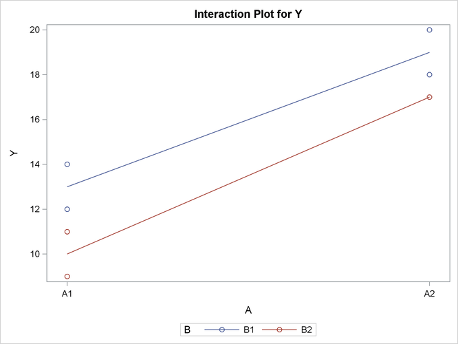
The insignificance of the A*B interaction is reflected in the fact that two lines in Figure 44.3 are nearly parallel. For more information about the graphics that GLM can produce, see the section ODS Graphics.