Algorithm and Notation :: SAS/STAT(R) 13.1 User's Guide

Algorithm and Notation

Subsections:

The PROFILE=, ROW=, and COLUMN= Options
The MCA Option
MCA Adjusted Inertias
Supplementary Rows and Columns
Statistics That Aid Interpretation

This section is primarily based on the theory of correspondence analysis found in Greenacre (1984). If you are interested in other references, see the section Background.

Let $\mb {N}$ be the contingency table formed from those observations and variables that are not supplementary and from those observations that have no missing values and have a positive weight. This table is an $(n_ r \times n_ c)$ rank q matrix of nonnegative numbers with nonzero row and column sums. If $\mb {Z}_ a$ is the binary coding for variable A, and $\mb {Z}_ b$ is the binary coding for variable B, then $\mb {N} = \mb {Z}_ a^\prime \mb {Z}_ b$ is a contingency table. Similarly, if $\mb {Z}_{b,c}$ contains the binary coding for both variables B and C, then $\mb {N} = \mb {Z}_ a^\prime \mb {Z}_{b,c}$ can also be input to a correspondence analysis. With the BINARY option, $\mb {N} = \mb {Z}$ , and the analysis is based on a binary table. In multiple correspondence analysis, the analysis is based on a Burt table, $\mb {Z}^\prime \mb {Z}$ .

Let $\mb {1}$ be a vector of 1s of the appropriate order, let $\mb {I}$ be an identity matrix, and let diag $(\cdot )$ be a matrix-valued function that creates a diagonal matrix from a vector. Let

$\begin{align*} f & = \mb {1^{\prime } N 1} \\ \mb {P} & = \frac{1}{f}\mb {N} \\ \mb {r} & = \mb {P1} \\ \mb {c} & = \mb {P^{\prime } 1} \\ \mb {D_ r} & = \mr {diag}(\mb {r}) \\ \mb {D_ c} & = \mr {diag}(\mb {c}) \\ \mb {R} & = \mb {D_ r^{-1} P} \\ \mb {C^{\prime }} & = \mb {D_ c^{-1} P^{\prime }} \\ \end{align*}$

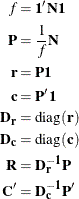
The scalar f is the sum of all elements in $\mb {N}$ . The matrix $\mb {P}$ is a matrix of relative frequencies. The vector $\mb {r}$ contains row marginal proportions or row “masses.” The vector $\mb {c}$ contains column marginal proportions or column masses. The matrices $\mb {D_ r}$ and $\mb {D_ c}$ are diagonal matrices of marginals.

The rows of $\mb {R}$ contain the “row profiles.” The elements of each row of $\mb {R}$ sum to one. Each $(i,j)$ element of $\mb {R}$ contains the observed probability of being in column j given membership in row i. Similarly, the columns of $\mb {C}$ contain the column profiles. The coordinates in correspondence analysis are based on the generalized singular value decomposition of $\mb {P}$ ,

$\mb {P} = \mb {A D_ u B^{\prime }}$

where

$\mb {A^{\prime } D_ r^{-1} A} = \mb {B^{\prime } D_ c^{-1} B} = \mb {I}$

In multiple correspondence analysis,

$\mb {P} = \mb {BD_ u^2B^{\prime }}$

The matrix $\mb {A}$ , which is the rectangular matrix of left generalized singular vectors, has $n_ r$ rows and q columns; the matrix $\mb {D_ u}$ , which is a diagonal matrix of singular values, has q rows and columns; and the matrix $\mb {B}$ , which is the rectangular matrix of right generalized singular vectors, has $n_ c$ rows and q columns. The columns of $\mb {A}$ and $\mb {B}$ define the principal axes of the column and row point clouds, respectively.

The generalized singular value decomposition of $\mb {P} - \mb {rc^{\prime }}$ , discarding the last singular value (which is zero) and the last left and right singular vectors, is exactly the same as a generalized singular value decomposition of $\mb {P}$ , discarding the first singular value (which is one), the first left singular vector, $\mb {r}$ , and the first right singular vector, $\mb {c}$ . The first (trivial) column of $\mb {A}$ and $\mb {B}$ and the first singular value in $\mb {D_ u}$ are discarded before any results are displayed. You can obtain the generalized singular value decomposition of $\mb {P} - \mb {rc}^{\prime }$ from the ordinary singular value decomposition of $\mb {D_ r^{-1/2}} (\mb {P} - \mb {rc}^\prime ) \mb {D_ c^{-1/2}}$ :

$\mb {D_ r^{-1/2}} (\mb {P} - \mb {rc}^\prime ) \mb {D_ c^{-1/2}} = \mb {U D_ u V}^\prime = (\mb {D_ r^{-1/2} A}) \mb {D_ u} (\mb {D_ c^{-1/2} B})^\prime$

$\mb {P} - \mb {rc}^\prime = \mb {D_ r^{1/2}} \mb {U D_ u V}^\prime \mb {D_ c^{1/2}} = \mb {(D_ r^{1/2}} \mb {U}) \mb {D_ u} (\mb {D_ c^{1/2}} \mb {V})^\prime = \mb {A D_ u B^{\prime }}$

Hence, $\mb {A} = \mb {D_ r^{1/2} U}$ and $\mb {B} = \mb {D_ c^{1/2} V}$ .

The default row coordinates are $\mb {D_ r^{-1}AD_ u}$ , and the default column coordinates are $\mb {D_ c^{-1}BD_ u}$ . Typically the first two columns of $\mb {D_ r^{-1}AD_ u}$ and $\mb {D_ c^{-1}BD_ u}$ are plotted to display graphically associations between the row and column categories. The plot consists of two overlaid plots, one for rows and one for columns. The row points are row profiles, and the column points are column profiles, both rescaled so that distances between profiles can be displayed as ordinary Euclidean distances, then orthogonally rotated to a principal axes orientation. Distances between row points and other row points have meaning, as do distances between column points and other column points. However, distances between column points and row points are not interpretable.

The PROFILE=, ROW=, and COLUMN= Options

The PROFILE=, ROW=, and COLUMN= options standardize the coordinates before they are displayed and placed in the output data set. The options PROFILE=BOTH, PROFILE=ROW, and PROFILE=COLUMN provide the standardizations that are typically used in correspondence analysis. There are six choices each for row and column coordinates (see Table 34.3). However, most of the combinations of the ROW= and COLUMN= options are not useful. The ROW= and COLUMN= options are provided for completeness, but they are not intended for general use.

Table 34.3: Coordinates

ROW=		Matrix Formula
A		$\mb {A}$
AD		$\mb {AD_ u}$
DA		$\mb {D_ r^{-1}A}$
DAD		$\mb {D_ r^{-1}AD_ u}$
DAD1/2		$\mb {D_ r^{-1}A} \mb {D_ u^{1/2}}$
DAID1/2		$\mb {D_ r^{-1}A}(\mb {I} + \mb {D_ u})^\mb {1/2}$
COLUMN=		Matrix Formula
B		$\mb {B}$
BD		$\mb {BD_ u}$
DB		$\mb {D_ c^{-1}B}$
DBD		$\mb {D_ c^{-1}BD_ u}$
DBD1/2		$\mb {D_ c^{-1}B} \mb {D_ u^{1/2}}$
DBID1/2		$\mb {D_ c^{-1}B}(\mb {I} + \mb {D_ u})^\mb {1/2}$

When PROFILE=ROW (ROW=DAD and COLUMN=DB), the row coordinates $\mb {D_ r^{-1}AD_ u}$ and column coordinates $\mb {D_ c^{-1}B}$ provide a correspondence analysis based on the row profile matrix. The row profile (conditional probability) matrix is defined as $\mb {R} = \mb {D_ r^{-1}P} = \mb {D_ r^{-1}AD_ uB^{\prime }}$ . The elements of each row of $\mb {R}$ sum to one. Each $(i,j)$ element of $\mb {R}$ contains the observed probability of being in column j given membership in row i. The “principal” row coordinates $\mb {D_ r^{-1}AD_ u}$ and “standard” column coordinates $\mb {D_ c^{-1}B}$ provide a decomposition of $\mb {D_ r^{-1}AD_ uB^{\prime }D_ c^{-1}} = \mb {D_ r^{-1}PD_ c^{-1}} = \mb {RD_ c^{-1}}$ . Because $\mb {D_ r^{-1}AD_ u} = \mb {RD_ c^{-1}B}$ , the row coordinates are weighted centroids of the column coordinates. Each column point, with coordinates scaled to standard coordinates, defines a vertex in $(n_ c-1)$ -dimensional space. All of the principal row coordinates are located in the space defined by the standard column coordinates. Distances among row points have meaning, but distances among column points and distances between row and column points are not interpretable.

The option PROFILE=COLUMN can be described as applying the PROFILE=ROW formulas to the transpose of the contingency table. When PROFILE=COLUMN (ROW=DA and COLUMN=DBD), the principal column coordinates $\mb {D_ c^{-1}BD_ u}$ are weighted centroids of the standard row coordinates $\mb {D_ r^{-1}A}$ . Each row point, with coordinates scaled to standard coordinates, defines a vertex in $(n_ r-1)$ -dimensional space. All of the principal column coordinates are located in the space defined by the standard row coordinates. Distances among column points have meaning, but distances among row points and distances between row and column points are not interpretable.

The usual sets of coordinates are given by the default PROFILE=BOTH (ROW=DAD and COLUMN=DBD). All of the summary statistics, such as the squared cosines and contributions to inertia, apply to these two sets of points. One advantage to using these coordinates is that both sets $(\mb {D_ r^{-1}AD_ u}$ and $\mb {D_ c^{-1}BD_ u})$ are postmultiplied by the diagonal matrix $\mb {D_ u}$ , which has diagonal values that are all less than or equal to one. When $\mb {D_ u}$ is a part of the definition of only one set of coordinates, that set forms a tight cluster near the centroid, whereas the other set of points is more widely dispersed. Including $\mb {D_ u}$ in both sets makes a better graphical display. However, care must be taken in interpreting such a plot. No correct interpretation of distances between row points and column points can be made.

Another property of this choice of coordinates concerns the geometry of distances between points within each set. The default row coordinates can be decomposed into $\mb {D_ r^{-1}AD_ u} = \mb {D_ r^{-1}AD_ uB^{\prime }D_ c^{-1}B} = (\mb {D_ r^{-1}P})(\mb {D_ c^{-1/2}})(\mb {D_ c^{-1/2}B})$ . The row coordinates are row profiles $(\mb {D_ r^{-1}P})$ , rescaled by $\mb {D_ c^{-1/2}}$ (rescaled so that distances between profiles are transformed from a chi-square metric to a Euclidean metric), then orthogonally rotated (with $\mb {D_ c^{-1/2}B}$ ) to a principal axes orientation. Similarly, the column coordinates are column profiles rescaled to a Euclidean metric and orthogonally rotated to a principal axes orientation.

The rationale for computing distances between row profiles by using the non-Euclidean chi-square metric is as follows. Each row of the contingency table can be viewed as a realization of a multinomial distribution conditional on its row marginal frequency. The null hypothesis of row and column independence is equivalent to the hypothesis of homogeneity of the row profiles. A significant chi-square statistic is geometrically interpreted as a significant deviation of the row profiles from their centroid, $\mb {c^{\prime }}$ . The chi-square metric is the Mahalanobis metric between row profiles based on their estimated covariance matrix under the homogeneity assumption (Greenacre and Hastie, 1987). A parallel argument can be made for the column profiles.

When ROW=DAD1/2 and COLUMN=DBD1/2 (Gifi, 1990; van der Heijden and de Leeuw, 1985), the row coordinates $\mb {D_ r^{-1}AD_ u^{1/2}}$ and column coordinates $\mb {D_ c^{-1}BD_ u^{1/2}}$ are a decomposition of $\mb {D_ r^{-1}PD_ c^{-1}}$ .

In all of the preceding pairs, distances between row and column points are not meaningful. This prompted Carroll, Green, and Schaffer (1986) to propose that row coordinates $\mb {D_ r^{-1}A}(\mb {I}+\mb {D_ u})^\mb {1/2}$ and column coordinates $\mb {D_ c^{-1}B}(\mb {I}+\mb {D_ u})^\mb {1/2}$ be used. These coordinates are (except for a constant scaling) the coordinates from a multiple correspondence analysis of a Burt table created from two categorical variables. This standardization is available with ROW=DAID1/2 and COLUMN=DBID1/2. However, this approach has been criticized on both theoretical and empirical grounds by Greenacre (1989). The Carroll, Green, and Schaffer standardization relies on the assumption that the chi-square metric is an appropriate metric for measuring the distance between the columns of a bivariate indicator matrix. See the section Using the TABLES Statement for a description of indicator matrices. Greenacre (1989) showed that this assumption cannot be justified.

The MCA Option

The MCA option performs a multiple correspondence analysis (MCA). This option requires a Burt table. You can specify the MCA option with a table created from a design matrix with fuzzy coding schemes as long as every row of every partition of the design matrix has the same marginal sum. For example, each row of each partition could contain the probabilities that the observation is a member of each level. Then the Burt table constructed from this matrix no longer contains all integers, and the diagonal partitions are no longer diagonal matrices, but MCA is still valid.

A TABLES statement with a single variable list creates a Burt table. Thus, you can always specify the MCA option with this type of input. If you use the MCA option when reading an existing table with a VAR statement, you must ensure that the table is a Burt table.

If you perform MCA on a table that is not a Burt table, the results of the analysis are invalid. If the table is not symmetric, or if the sums of all elements in each diagonal partition are not equal, PROC CORRESP displays an error message and quits.

A subset of the columns of a Burt table is not necessarily a Burt table, so in MCA it is not appropriate to designate arbitrary columns as supplementary. You can, however, designate all columns from one or more categorical variables as supplementary.

The results of a multiple correspondence analysis of a Burt table $\mb {Z}^\prime \mb {Z}$ are the same as the column results from a simple correspondence analysis of the binary (or fuzzy) matrix $\mb {Z}$ . Multiple correspondence analysis is not a simple correspondence analysis of the Burt table. It is not appropriate to perform a simple correspondence analysis of a Burt table. The MCA option is based on $\mb {P} = \mb {BD_ u^2B^{\prime }}$ , whereas a simple correspondence analysis of the Burt table would be based on $\mb {P} = \mb {BD_ uB^{\prime }}$ .

Because the rows and columns of the Burt table are the same, no row information is displayed or written to the output data sets. The resulting inertias and the default (COLUMN=DBD) column coordinates are the appropriate inertias and coordinates for an MCA. The supplementary column coordinates, cosines, and quality of representation formulas for MCA differ from the simple correspondence analysis formulas because the design matrix column profiles and left singular vectors are not available.

The following statements create a Burt table and perform a multiple correspondence analysis:

proc corresp data=Neighbor observed short mca;
   tables Hair Height Sex Age;
run;

Both the rows and the columns have the same nine categories (Blond, Brown, White, Short, Tall, Female, Male, Old, and Young).

MCA Adjusted Inertias

The usual principal inertias of a Burt table constructed from m categorical variables in MCA are the eigenvalues $u_ k$ from $\mb {D_ u^2}$ . The problem with these inertias is that they provide a pessimistic indication of fit. Benzécri (1979) proposed the following inertia adjustment, which is also described by Greenacre (1984, p. 145):

$\left(\frac{m}{m - 1}\right)^2 \times \left(u_ k - \frac{1}{m}\right)^2$ $~ ~ ~ ~ ~ ~ ~ ~$ for $u_ k > \frac{1}{m}$

This adjustment computes the percent of adjusted inertia relative to the sum of the adjusted inertias for all inertias greater than $\frac{1}{m}$ . The Benzécri adjustment is available with the BENZECRI option.

Greenacre (1994, p. 156) argues that the Benzécri adjustment overestimates the quality of fit. Greenacre proposes instead to compute the percentage of adjusted inertia relative to

$\frac{m}{m - 1} \left(\hbox{trace}({D_ u^4}) - \frac{n_ c - m}{m^2}\right)$

for all inertias greater than $\frac{1}{m}$ , where $\hbox{trace}({D_ u^4})$ is the sum of squared inertias. The Greenacre adjustment is available with the GREENACRE option.

Ordinary unadjusted inertias are printed by default with MCA when neither the BENZECRI nor the GREENACRE option is specified. However, the unadjusted inertias are not printed by default when either the BENZECRI or the GREENACRE option is specified. To display both adjusted and unadjusted inertias, specify the UNADJUSTED option in addition to the relevant adjusted inertia option (BENZECRI, GREENACRE, or both).

Supplementary Rows and Columns

Supplementary rows and columns are represented as points in the joint row and column space, but they are not used in determining the locations of the other active rows and columns of the table. The formulas that are used to compute coordinates for the supplementary rows and columns depend on the PROFILE= option or the ROW= and COLUMN= options. Let $\mb {S_ o}$ be a matrix with rows that contain the supplementary observations, and let $\mb {S_ v}$ be a matrix with rows that contain the supplementary variables. Note that $\mb {S_ v}$ is defined to be the transpose of the supplementary variable partition of the table. Let $\mb {R_ s} = \mr {diag}(\mb {S_ o1})^\mb {-1}\mb {S_ o}$ be the supplementary observation profile matrix, and let $\mb {C_ s} = \mr {diag}(\mb {S_ v1})^\mb {-1}\mb {S_ v}$ be the supplementary variable profile matrix. Note that the notation diag $(\cdot )^\mb {-1}$ means to convert the vector to a diagonal matrix, then invert the diagonal matrix. The coordinates for the supplementary observations and variables are shown in Table 34.4.

Table 34.4: Coordinates for Supplementary Observations

ROW=	Matrix Formula
A	$\frac{1}{f}\mb {S_ oD_ c^{-1}BD_ u^{-1}}$
AD	$\frac{1}{f}\mb {S_ oD_ c^{-1}B}$
DA	$\mb {R_ sD_ c^{-1}BD_ u^{-1}}$
DAD	$\mb {R_ sD_ c^{-1}B}$
DAD1/2	$\mb {R_ sD_ c^{-1}BD_ u^{-1/2}}$
DAID1/2	$\mb {R_ sD_ c^{-1}BD_ u^{-1}}(\mb {I} + \mb {D_ u})^\mb {1/2}$
COLUMN=	Matrix Formula
B	$\frac{1}{f}\mb {S_ vD_ r^{-1}AD_ u^{-1}}$
BD	$\frac{1}{f}\mb {S_ vD_ r^{-1}A}$
DB	$\mb {C_ sD_ r^{-1}AD_ u^{-1}}$
DBD	$\mb {C_ sD_ r^{-1}A}$
DBD1/2	$\mb {C_ sD_ r^{-1}AD_ u^{-1/2}}$
DBID1/2	$\mb {C_ sD_ r^{-1}AD_ u^{-1}}(\mb {I} + \mb {D_ u})^\mb {1/2}$
MCA COLUMN=	Matrix Formula
B	not allowed
BD	not allowed
DB	$\mb {C_ sD_ r^{-1}BD_ u^{-2}}$
DBD	$\mb {C_ sD_ r^{-1}BD_ u^{-1}}$
DBD1/2	$\mb {C_ sD_ r^{-1}BD_ u^{-3/2}}$
DBID1/2	$\mb {C_ sD_ r^{-1}BD_ u^{-2}}(\mb {I} + \mb {D_ u})^\mb {1/2}$

Statistics That Aid Interpretation

The partial contributions to inertia, squared cosines, quality of representation, inertia, and mass provide additional information about the coordinates. These statistics are displayed by default. Include the SHORT or NOPRINT option in the PROC CORRESP statement to avoid having these statistics displayed.

These statistics pertain to the default PROFILE=BOTH coordinates, no matter what values you specify for the ROW=, COLUMN=, or PROFILE= option. Let $\mr {sq}(\cdot )$ be a matrix-valued function denoting element-wise squaring of the argument matrix. Let t be the total inertia (the sum of the elements in $\mb {D_ u^2}$ ).

In MCA, let $\mb {D_ s}$ be the Burt table partition containing the intersection of the supplementary columns and the supplementary rows. The matrix $\mb {D_ s}$ is a diagonal matrix of marginal frequencies of the supplemental columns of the binary matrix $\mb {Z}$ . Let p be the number of rows in this design matrix. The statistics are defined in Table 34.5.

Table 34.5: Statistics That Aid Interpretation

Statistic		Matrix Formula
Row partial contributions		$\mb {D_ r^{-1}}\mr {sq}(\mb {A})$
to inertia
Column partial contributions		$\mb {D_ c^{-1}}\mr {sq}(\mb {B})$
to inertia
Row squared cosines		$\mr {diag}(\mr {sq}(\mb {AD_ u}) \mb {1})^\mb {-1}\mr {sq}(\mb {AD_ u})$
Column squared cosines		$\mr {diag}(\mr {sq}(\mb {BD_ u}) \mb {1})^\mb {-1}\mr {sq}(\mb {BD_ u})$
Row mass		$\mb {r}$
Column mass		$\mb {c}$
Row inertia		$\frac{1}{t}\mb {D_ r^{-1}}\mr {sq}(\mb {AD_ u})\mb {1}$
Column inertia		$\frac{1}{t}\mb {D_ c^{-1}}\mr {sq}(\mb {BD_ u})\mb {1}$
Supplementary row		$\mr {diag}(\mr {sq}(\mb {R_ s}-\mb {1c^{\prime }}) \mb {D_ c^{-1}1})^\mb {-1}\mr {sq}(\mb {R_ sD_ c^{-1}B})$
squared cosines
Supplementary column		$\mr {diag}(\mr {sq}(\mb {C_ s}-\mb {1r^{\prime }}) \mb {D_ r^{-1}1})^\mb {-1}\mr {sq}(\mb {C_ sD_ r^{-1}A})$
squared cosines
MCA supplementary column		$\mb {D_ s}(p\mb {I-D_ s})^\mb {-1} \mr {sq}(\mb {C_ sD_ r^{-1}BD_ u^{-1}})$
squared cosines

The quality of representation in the DIMENS=n dimensional display of any point is the sum of its squared cosines over only the n dimensions. Inertia and mass are not defined for supplementary points.

A table that summarizes the partial contributions to inertia table is also computed. The points that best explain the inertia of each dimension and the dimension to which each point contributes the most inertia are indicated. The output data set variable names for this table are Best1–Bestn (where DIMENS=n) and Best. The Best column contains the dimension number of the largest partial contribution to inertia for each point (the index of the maximum value in each row of $\mb {D_ r^{-1}}\mr {sq}(\mb {A})$ or $\mb {D_ c^{-1}}\mr {sq}(\mb {B})$ ).

For each row, the Best1–Bestn columns contain either the corresponding value of Best, if the point is one of the biggest contributors to the dimension’s inertia, or 0 if it is not. Specifically, Best1 contains the value of Best for the point with the largest contribution to dimension one’s inertia. A cumulative proportion sum is initialized to this point’s partial contribution to the inertia of dimension one. If this sum is less than the value for the MININERTIA= option, then Best1 contains the value of Best for the point with the second-largest contribution to dimension one’s inertia. Otherwise, this point’s Best1 is 0. This point’s partial contribution to inertia is added to the sum. This process continues for the point with the third-largest partial contribution, and so on, until adding a point’s contribution to the sum increases the sum beyond the value of the MININERTIA= option. This same algorithm is then used for Best2, and so on.

For example, the following table contains contributions to inertia and the corresponding Best variables. The contribution to inertia variables are proportions that sum to 1 within each column. The first point makes its greatest contribution to the inertia of dimension two, so Best for point one is set to 2, and Best1–Best3 for point one must all be 0 or 2. The second point also makes its greatest contribution to the inertia of dimension two, so Best for point two is set to 2, and Best1–Best3 for point two must all be 0 or 2, and so on.

Assume MININERTIA=0.8, the default. Table 34.6 shows some contributions to inertia. In dimension one, the largest contribution is 0.41302 for the fourth point, so Best1 is set to 1, the value of Best for the fourth point. Because this value is less than 0.8, the second-largest value (0.36456 for point five) is found and its Best1 is set to its Best’s value of 1. Because $0.41302 + 0.36456 = 0.77758$ is less than 0.8, the third point (0.0882 at point eight) is found and Best1 is set to 3, because the contribution to dimension three for that point is greater than the contribution to dimension one. This increases the sum of the partial contributions to greater than 0.8, so the remaining Best1 values are all 0.

Table 34.6: Best Statistics

`Contr1`	`Contr2`	`Contr3`	`Best1`	`Best2`	`Best3`	`Best`
0.01593	0.32178	0.07565	0	2	2	2
0.03014	0.24826	0.07715	0	2	2	2
0.00592	0.02892	0.02698	0	0	0	2
0.41302	0.05191	0.05773	1	0	0	1
0.36456	0.00344	0.15565	1	0	1	1
0.03902	0.30966	0.11717	0	2	2	2
0.00019	0.01840	0.00734	0	0	0	2
0.08820	0.00527	0.16555	3	0	3	3
0.01447	0.00024	0.03851	0	0	0	3
0.02855	0.01213	0.27827	0	0	3	3

The CORRESP Procedure