Example 99.3 Paired Comparisons :: SAS/STAT(R) 12.3 User's Guide

Example 99.3 Paired Comparisons

When it is not feasible to assume that two groups of data are independent, and a natural pairing of the data exists, it is advantageous to use an analysis that takes the correlation into account. Using this correlation results in higher power to detect existing differences between the means. The differences between paired observations are assumed to be normally distributed. Some examples of this natural pairing are as follows:

pre- and post-test scores for a student receiving tutoring
fuel efficiency readings of two fuel types observed on the same automobile
sunburn scores for two sunblock lotions, one applied to the individual’s right arm, one to the left arm
political attitude scores of husbands and wives

In this example, taken from the SUGI Supplemental Library User’s Guide, Version 5 Edition, a stimulus is being examined to determine its effect on systolic blood pressure. Twelve men participate in the study. Each man’s systolic blood pressure is measured both before and after the stimulus is applied. The following statements input the data:

data pressure;
   input SBPbefore SBPafter @@;
   datalines;
120 128   124 131   130 131   118 127
140 132   128 125   140 141   135 137
126 118   130 132   126 129   127 135
;

The variables SBPbefore and SBPafter denote the systolic blood pressure before and after the stimulus, respectively.

The statements to perform the test follow:

ods graphics on;

proc ttest;
   paired SBPbefore*SBPafter;
run;

ods graphics off;

The PAIRED statement is used to test whether the mean change in systolic blood pressure is significantly different from zero. The tabular output is displayed in Output 99.3.1.

Output 99.3.1: TTEST Results

The TTEST Procedure

Difference: SBPbefore - SBPafter

N	Mean	Std Dev	Std Err	Minimum	Maximum
12	-1.8333	5.8284	1.6825	-9.0000	8.0000

Mean	95% CL Mean		Std Dev	95% CL Std Dev
-1.8333	-5.5365	1.8698	5.8284	4.1288	9.8958

DF	t Value	Pr > \|t\|
11	-1.09	0.2992

The variables SBPbefore and SBPafter are the paired variables with a sample size of 12. The summary statistics of the difference are displayed (mean, standard deviation, and standard error) along with their confidence limits. The minimum and maximum differences are also displayed. The t test is not significant (t = –1.09, p = 0.2992), indicating that the stimuli did not significantly affect systolic blood pressure.

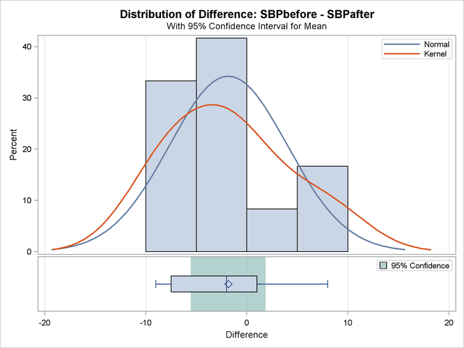
The summary panel in Output 99.3.2 shows a histogram, normal and kernel densities, box plot, and $100(1-\alpha )\% = 95\%$ confidence interval of the SBPbefore – SBPafter difference.

Output 99.3.2: Summary Panel

The agreement plot in Output 99.3.3 reveals that only three men have higher blood pressure before the stimulus than after.

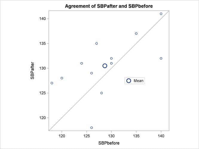
Output 99.3.3: Agreement of Treatments

But the differences for these men are relatively large, keeping the mean difference only slightly negative.

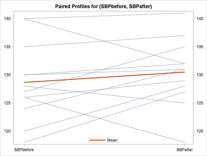
The profiles plot in Output 99.3.4 is a different view of the same information contained in Output 99.3.3, plotting the blood pressure from before to after the stimulus.

Output 99.3.4: Profiles over Treatments

The Q-Q plot in Output 99.3.5 assesses the normality assumption.

Output 99.3.5: Q-Q Plot

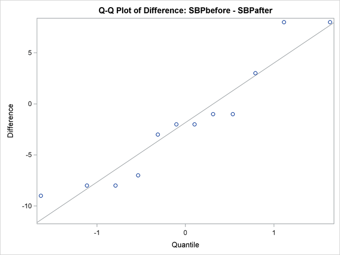
The Q-Q plot shows no obvious deviations from normality. You can check the assumption of normality more rigorously by using PROC UNIVARIATE with the NORMAL option.