The PRINCOMP Procedure

This example uses the PRINCOMP procedure to analyze job performance. Police officers were rated by their supervisors in 14 categories as part of standard police departmental administrative procedure.
The following statements create the Jobratings data set:
options validvarname=any;
data Jobratings;
   input 'Communication Skills'n         'Problem Solving'n
         'Learning Ability'n             'Judgment Under Pressure'n
         'Observational Skills'n         'Willingness to Confront Problems'n
         'Interest in People'n           'Interpersonal Sensitivity'n
         'Desire for Self-Improvement'n  'Appearance'n
         'Dependability'n                'Physical Ability'n
         'Integrity'n                    'Overall Rating'n;
   datalines;
2 6 8 3 8 8 5 3 8 7 9 8 6 7 7 4 7 5 8 8 7 6 8 5 7 6 6 7 5 6 7 5 7 8 6 3 7 7 5
8 7 5 6 7 8 6 9 7 7 7 9 8 8 9 9 7 9 9 9 9 7 7 9 8 8 7 8 8 8 8 8 9 8 9 7 8 9 9
8 8 8 7 9 9 8 9 9 9 9 8 8 9 8 9 9 7 9 8 8 7 7 9 4 7 9 8 4 6 8 8 8 6 3 5 6 5 2

   ... more lines ...

7 8 9 9 7 9 9 7 9 9 9 9 8 9 9 8 9 9 8 9 9 8 9 9 7 6 6 5 6 3 9 9 5 6 7 4 8 6
;
The data set Jobratings contains 14 variables. Each variable contains the job ratings, using a scale measurement from 1 to 10 (1=fail to comply,
10=exceptional). The last variable Overall Rating contains a score as an overall index on how each officer performs.
The following statements request a principal component analysis on the Jobratings data set, output the scores to the Scores data set (OUT= Scores), and produce default plots. Note that variable Overall Rating is excluded from the analysis.
ods graphics on;

proc princomp data=Jobratings(drop='Overall Rating'n);
run;
Output 73.3.1 and Output 73.3.2 display the PROC PRINCOMP output, beginning with simple statistics followed by the correlation matrix. By default, the PROC
PRINCOMP statement requests principal components computed from the correlation matrix, so the total variance is equal to the
number of variables, 13. In this example, it would also be reasonable to use the COV option, which would cause variables with
a high variance (such as Dependability) to have more influence on the results than variables with a low variance (such as Learning Ability). If you used the COV option, scores would be computed from centered rather than standardized variables.
Output 73.3.1: Simple Statistics and Correlation Matrix from the PRINCOMP Procedure
| Observations | 37 |
|---|---|
| Variables | 13 |
| Simple Statistics | |||||||||||||
|---|---|---|---|---|---|---|---|---|---|---|---|---|---|
| Communication Skills | Problem Solving | Learning Ability | Judgment Under Pressure | Observational Skills | Willingness to Confront Problems |
Interest in People | Interpersonal Sensitivity | Desire for Self-Improvement | Appearance | Dependability | Physical Ability | Integrity | |
| Mean | 6.567567568 | 6.675675676 | 6.891891892 | 6.378378378 | 7.081081081 | 6.756756757 | 6.675675676 | 6.540540541 | 7.027027027 | 7.135135135 | 7.027027027 | 7.162162162 | 7.081081081 |
| StD | 1.878837414 | 1.748873511 | 1.696135866 | 2.252792728 | 1.816259563 | 2.126622327 | 1.871631108 | 2.218540494 | 1.707605316 | 1.436859271 | 1.499749729 | 1.343988953 | 1.460182226 |
| Correlation Matrix | |||||||||||||
|---|---|---|---|---|---|---|---|---|---|---|---|---|---|
| Communication Skills |
Problem Solving | Learning Ability | Judgment Under Pressure |
Observational Skills |
Willingness to Confront Problems |
Interest in People |
Interpersonal Sensitivity |
Desire for Self-Improvement |
Appearance | Dependability | Physical Ability | Integrity | |
| Communication Skills | 1.0000 | 0.7254 | 0.3685 | 0.6107 | 0.4338 | 0.5708 | 0.4646 | 0.2975 | 0.0211 | -.0086 | -.2619 | -.1145 | -.2096 |
| Problem Solving | 0.7254 | 1.0000 | 0.6715 | 0.6877 | 0.6207 | 0.6504 | 0.3828 | 0.3113 | 0.1890 | 0.1064 | -.0389 | -.0361 | -.1852 |
| Learning Ability | 0.3685 | 0.6715 | 1.0000 | 0.5126 | 0.7603 | 0.3545 | 0.1024 | 0.3112 | 0.3079 | 0.1885 | 0.0121 | 0.0932 | -.1085 |
| Judgment Under Pressure | 0.6107 | 0.6877 | 0.5126 | 1.0000 | 0.5761 | 0.6227 | 0.5635 | 0.4915 | 0.1489 | 0.1382 | -.1347 | -.1217 | -.1025 |
| Observational Skills | 0.4338 | 0.6207 | 0.7603 | 0.5761 | 1.0000 | 0.4655 | 0.2449 | 0.4921 | 0.4113 | 0.0915 | -.1640 | 0.0741 | -.0549 |
| Willingness to Confront Problems | 0.5708 | 0.6504 | 0.3545 | 0.6227 | 0.4655 | 1.0000 | 0.4751 | 0.2170 | 0.1931 | 0.1111 | 0.2286 | 0.1114 | -.1813 |
| Interest in People | 0.4646 | 0.3828 | 0.1024 | 0.5635 | 0.2449 | 0.4751 | 1.0000 | 0.5652 | 0.3765 | 0.2750 | 0.1220 | 0.0215 | 0.1115 |
| Interpersonal Sensitivity | 0.2975 | 0.3113 | 0.3112 | 0.4915 | 0.4921 | 0.2170 | 0.5652 | 1.0000 | 0.5460 | 0.4121 | 0.0790 | 0.1747 | 0.1747 |
| Desire for Self-Improvement | 0.0211 | 0.1890 | 0.3079 | 0.1489 | 0.4113 | 0.1931 | 0.3765 | 0.5460 | 1.0000 | 0.5645 | 0.2166 | 0.3248 | 0.3667 |
| Appearance | -.0086 | 0.1064 | 0.1885 | 0.1382 | 0.0915 | 0.1111 | 0.2750 | 0.4121 | 0.5645 | 1.0000 | 0.5525 | 0.3479 | 0.4183 |
| Dependability | -.2619 | -.0389 | 0.0121 | -.1347 | -.1640 | 0.2286 | 0.1220 | 0.0790 | 0.2166 | 0.5525 | 1.0000 | 0.5628 | 0.3415 |
| Physical Ability | -.1145 | -.0361 | 0.0932 | -.1217 | 0.0741 | 0.1114 | 0.0215 | 0.1747 | 0.3248 | 0.3479 | 0.5628 | 1.0000 | 0.5027 |
| Integrity | -.2096 | -.1852 | -.1085 | -.1025 | -.0549 | -.1813 | 0.1115 | 0.1747 | 0.3667 | 0.4183 | 0.3415 | 0.5027 | 1.0000 |
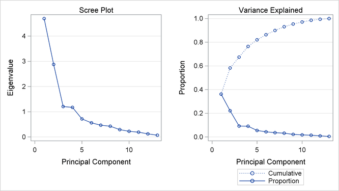
Output 73.3.2 displays the eigenvalues. The first principal component explains about 50% of the total variance, the second principal component explains about 13.6%, and the third principal component explains about 7.7%. Note that the eigenvalues sum to the total variance. The eigenvalues indicate that three to five components provide a good summary of the data, with three components accounting for about 71.7% of the total variance and five components explaining about 82.7%. Subsequent components contribute less than 5% each.
Output 73.3.2: Eigenvalues and Eigenvectors from the PRINCOMP Procedure
| Eigenvalues of the Correlation Matrix | ||||
|---|---|---|---|---|
| Eigenvalue | Difference | Proportion | Cumulative | |
| 1 | 4.69468687 | 1.81899683 | 0.3611 | 0.3611 |
| 2 | 2.87569003 | 1.67100277 | 0.2212 | 0.5823 |
| 3 | 1.20468727 | 0.03118935 | 0.0927 | 0.6750 |
| 4 | 1.17349791 | 0.45846322 | 0.0903 | 0.7653 |
| 5 | 0.71503470 | 0.15713583 | 0.0550 | 0.8203 |
| 6 | 0.55789887 | 0.09269082 | 0.0429 | 0.8632 |
| 7 | 0.46520805 | 0.04118763 | 0.0358 | 0.8990 |
| 8 | 0.42402041 | 0.13454552 | 0.0326 | 0.9316 |
| 9 | 0.28947489 | 0.06869311 | 0.0223 | 0.9539 |
| 10 | 0.22078178 | 0.03221769 | 0.0170 | 0.9708 |
| 11 | 0.18856410 | 0.06620108 | 0.0145 | 0.9853 |
| 12 | 0.12236302 | 0.05427092 | 0.0094 | 0.9948 |
| 13 | 0.06809210 | 0.0052 | 1.0000 | |
| Eigenvectors | |||||||||||||
|---|---|---|---|---|---|---|---|---|---|---|---|---|---|
| Prin1 | Prin2 | Prin3 | Prin4 | Prin5 | Prin6 | Prin7 | Prin8 | Prin9 | Prin10 | Prin11 | Prin12 | Prin13 | |
| Communication Skills | 0.323548 | -.236730 | 0.206727 | 0.092655 | 0.293138 | 0.260352 | -.215988 | -.550645 | -.050648 | 0.107002 | 0.262509 | 0.341232 | 0.291574 |
| Problem Solving | 0.383857 | -.160898 | -.091224 | 0.212751 | 0.025258 | 0.252518 | -.140816 | -.104392 | 0.283104 | 0.221940 | -.548010 | -.492803 | -.073999 |
| Learning Ability | 0.322899 | -.050464 | -.553565 | 0.056656 | -.138393 | 0.168405 | 0.150062 | 0.055518 | 0.391053 | -.223399 | 0.132338 | 0.442471 | -.307096 |
| Judgment Under Pressure | 0.379958 | -.142821 | 0.155157 | -.025467 | 0.043612 | 0.175269 | 0.361045 | 0.391055 | -.315796 | -.392714 | -.286021 | 0.111225 | 0.382730 |
| Observational Skills | 0.359246 | -.067434 | -.424397 | -.148191 | 0.093417 | -.221005 | 0.022944 | 0.177808 | -.141401 | 0.225326 | 0.502509 | -.416669 | 0.278776 |
| Willingness to Confront Problems | 0.333754 | -.064285 | 0.183338 | 0.459764 | -.024447 | -.304704 | -.247094 | 0.259896 | -.387665 | 0.158552 | 0.047611 | 0.168464 | -.459746 |
| Interest in People | 0.296160 | 0.082187 | 0.575827 | -.140226 | 0.023973 | -.159653 | -.015476 | 0.131682 | 0.540942 | -.277206 | 0.299254 | -.197252 | -.112818 |
| Interpersonal Sensitivity | 0.302693 | 0.180810 | 0.119231 | -.432281 | -.047507 | -.238610 | 0.501550 | -.303435 | -.097727 | 0.393688 | -.196906 | 0.137833 | -.222427 |
| Desire for Self-Improvement | 0.225795 | 0.344251 | -.123236 | -.333516 | -.174557 | -.266896 | -.621875 | 0.020842 | 0.018350 | -.105222 | -.293349 | 0.219662 | 0.263644 |
| Appearance | 0.158341 | 0.425329 | 0.052469 | -.022665 | -.441729 | 0.494677 | -.051864 | -.204081 | -.350816 | -.186793 | 0.226289 | -.256802 | -.177399 |
| Dependability | 0.025597 | 0.427337 | 0.079019 | 0.520679 | -.289013 | -.044047 | 0.221520 | 0.079762 | 0.250326 | 0.336689 | 0.049300 | 0.146711 | 0.445532 |
| Physical Ability | 0.052980 | 0.418985 | -.185687 | 0.312555 | 0.486621 | -.299641 | 0.145579 | -.340453 | -.072184 | -.432711 | -.090520 | -.154868 | -.034075 |
| Integrity | -.006172 | 0.435225 | 0.015874 | -.147905 | 0.578186 | 0.421421 | -.087126 | 0.396179 | 0.030130 | 0.284351 | 0.021483 | 0.113790 | -.129601 |
PROC PRINCOMP produces the scree plot as shown in Output 73.3.3 by default when ODS Graphics is enabled. You can obtain more plots by specifying the PLOTS= option in the PROC PRINCOMP statement.
The “Scree Plot” on the left shows that the eigenvalue of the first component is approximately 6.5 and the eigenvalue of the second component is largely decreased to under 2.0. The “Variance Explained” plot on the right shows that you can explain a near 80% of total variance with the first four principal components.
The first component reflects overall performance since the first eigenvector shows approximately equal loadings on all variables.
The second eigenvector has high positive loadings on the variables Observational Skills and Willingness to Confront Problems but even higher negative loadings on the variables Interest in People and Interpersonal Sensitivity. This component seems to reflect the ability to take action, but it also reflects a lack of interpersonal skills. The third
eigenvector has a very high positive loading on the variable Physical Ability and high negative loadings on the variables Problem Solving and Learning Ability. This component seems to reflect physical strength, but also shows poor learning and problem-solving skills.
In short, the three components represent the following:
- First Component:
-
overall performance
- Second Component:
-
smart, tough, and introverted
- Third Component:
-
superior strength and average intellect
PROC PRINCOMP also produces other plots besides the scree plot, which are helpful while interpreting the results. The following statements request plots from the PRINCOMP procedure:
proc princomp data=Jobratings(drop='Overall Rating'n)
              plots(ncomp=3)=all n=5;
run;
PLOTS=ALL(NCOMP=3) in the PROC PRINCOMP statement requests all plots to be produced but limits the number of components to be plotted in the component pattern plots and the component score plots to three. The N=5 option sets the number of principal components to be computed to five. Besides a scree plot similar to the one shown before, the rest of plots are displayed in the following context.
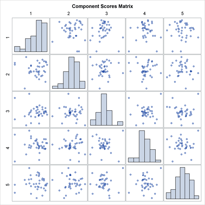
Output 73.3.4 shows a matrix plot of component scores between the first five principal components. The histogram of each component is displayed in the diagonal element of the matrix. The histograms indicate that the first principal component is skewed to the left and the second principal component is slightly skewed to the right.
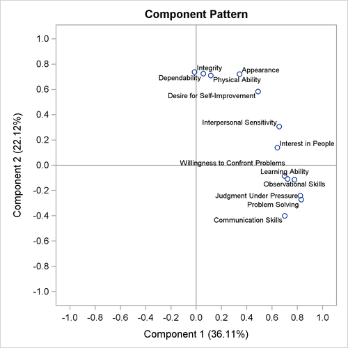
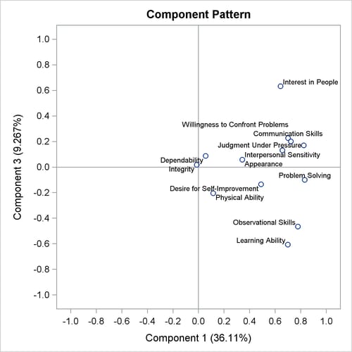
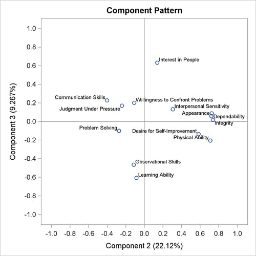
The pairwise component pattern plots are shown in Output 73.3.5 to Output 73.3.7. The pattern plots show the following:
-
All variables positively and evenly correlate with the first principal component (Output 73.3.5 and Output 73.3.6).
-
The variables
Observational SkillsandWillingness to Confront Problemscorrelate highly with the second component, and the variablesInterest in PeopleandInterpersonal Sensitivitycorrelate highly but negatively with the second component (Output 73.3.5). -
The variable
Physical Abilitycorrelates highly with the third component, and the variablesProblem SolvingandLearning Abilitycorrelate highly but negatively with the third component (Output 73.3.6). -
The variable
Observational Skills,Willingness to Confront Problems,Interest in People, andInterpersonal Sensitivitycorrelate highly (either positively or negatively) with the second component, but all have very low correlations with the third component; the variablesPhysical AbilityandProblem Solvingcorrelate highly (either positively or negatively) with the third component, but both have very low correlations with the second component (Output 73.3.7).
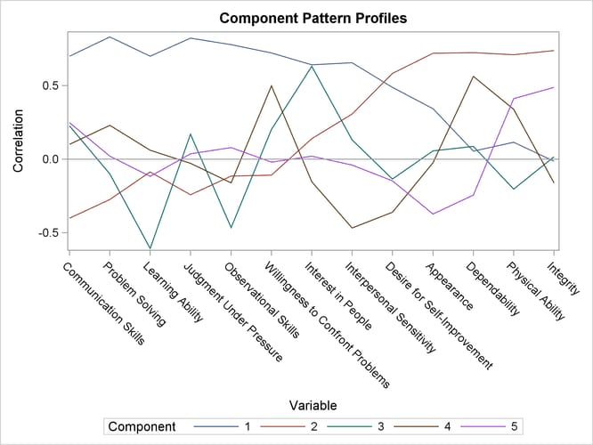
Output 73.3.8 shows a component pattern profile. As it was shown in the pattern plots, the nearly horizontal profile from the first component indicates that the first component is mostly correlated evenly across all variables.
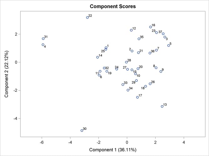
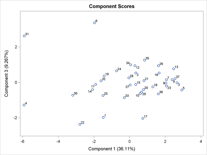
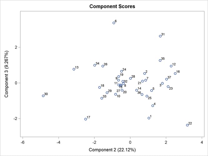
Output 73.3.9 through Output 73.3.11 display the pairwise component score plots. Observation numbers are used as the plotting symbol.
Output 73.3.9 shows a scatter plot of the first and third components. Observations 82, 9, and 84 seem like outliers on the first component; Observations 16 and 59 can be potential outliers on the second component.
Output 73.3.10 shows a scatter plot of the first and third components. Observations 82, 9, and 84 seem like outliers on the first component.
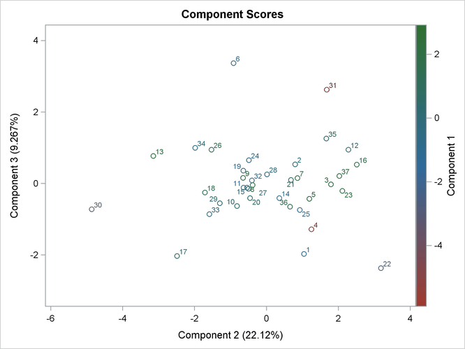
Output 73.3.11 shows a scatter plot of the second and third components. Observations 95, 15, 16, and 59 can be potential outliers on the second component.
Output 73.3.12 shows a scatter plot of the second and third components, displaying the first component with color. Color interpolation in the HTMLBLUE style ranges from red (minimum) to blue (middle) and to green (maximum).