Example 70.1 Examining Model Details :: SAS/STAT(R) 12.3 User's Guide

Example 70.1 Examining Model Details

This example, from Umetrics (1995), demonstrates different ways to examine a PLS model. The data come from the field of drug discovery. New drugs are developed from chemicals that are biologically active. Testing a compound for biological activity is an expensive procedure, so it is useful to be able to predict biological activity from cheaper chemical measurements. In fact, computational chemistry makes it possible to calculate certain chemical measurements without even making the compound. These measurements include size, lipophilicity, and polarity at various sites on the molecule. The following statements create a data set named pentaTrain, which contains these data.

data pentaTrain;
   input obsnam $ S1 L1 P1 S2 L2 P2
                  S3 L3 P3 S4 L4 P4
                  S5 L5 P5  log_RAI @@;
   n = _n_;
   datalines;
VESSK    -2.6931 -2.5271 -1.2871  3.0777  0.3891 -0.0701
          1.9607 -1.6324  0.5746  1.9607 -1.6324  0.5746
          2.8369  1.4092 -3.1398                    0.00
VESAK    -2.6931 -2.5271 -1.2871  3.0777  0.3891 -0.0701
          1.9607 -1.6324  0.5746  0.0744 -1.7333  0.0902
          2.8369  1.4092 -3.1398                    0.28
VEASK    -2.6931 -2.5271 -1.2871  3.0777  0.3891 -0.0701
          0.0744 -1.7333  0.0902  1.9607 -1.6324  0.5746
          2.8369  1.4092 -3.1398                    0.20
VEAAK    -2.6931 -2.5271 -1.2871  3.0777  0.3891 -0.0701
          0.0744 -1.7333  0.0902  0.0744 -1.7333  0.0902
          2.8369  1.4092 -3.1398                    0.51
VKAAK    -2.6931 -2.5271 -1.2871  2.8369  1.4092 -3.1398
          0.0744 -1.7333  0.0902  0.0744 -1.7333  0.0902
          2.8369  1.4092 -3.1398                    0.11
VEWAK    -2.6931 -2.5271 -1.2871  3.0777  0.3891 -0.0701
         -4.7548  3.6521  0.8524  0.0744 -1.7333  0.0902
          2.8369  1.4092 -3.1398                    2.73
VEAAP    -2.6931 -2.5271 -1.2871  3.0777  0.3891 -0.0701
          0.0744 -1.7333  0.0902  0.0744 -1.7333  0.0902
         -1.2201  0.8829  2.2253                    0.18
VEHAK    -2.6931 -2.5271 -1.2871  3.0777  0.3891 -0.0701
          2.4064  1.7438  1.1057  0.0744 -1.7333  0.0902
          2.8369  1.4092 -3.1398                    1.53
VAAAK    -2.6931 -2.5271 -1.2871  0.0744 -1.7333  0.0902
          0.0744 -1.7333  0.0902  0.0744 -1.7333  0.0902
          2.8369  1.4092 -3.1398                   -0.10
GEAAK     2.2261 -5.3648  0.3049  3.0777  0.3891 -0.0701
          0.0744 -1.7333  0.0902  0.0744 -1.7333  0.0902
          2.8369  1.4092 -3.1398                   -0.52
LEAAK    -4.1921 -1.0285 -0.9801  3.0777  0.3891 -0.0701
          0.0744 -1.7333  0.0902  0.0744 -1.7333  0.0902
          2.8369  1.4092 -3.1398                    0.40
FEAAK    -4.9217  1.2977  0.4473  3.0777  0.3891 -0.0701
          0.0744 -1.7333  0.0902  0.0744 -1.7333  0.0902
          2.8369  1.4092 -3.1398                    0.30
VEGGK    -2.6931 -2.5271 -1.2871  3.0777  0.3891 -0.0701
          2.2261 -5.3648  0.3049  2.2261 -5.3648  0.3049
          2.8369  1.4092 -3.1398                   -1.00
VEFAK    -2.6931 -2.5271 -1.2871  3.0777  0.3891 -0.0701
         -4.9217  1.2977  0.4473  0.0744 -1.7333  0.0902
          2.8369  1.4092 -3.1398                    1.57
VELAK    -2.6931 -2.5271 -1.2871  3.0777  0.3891 -0.0701
         -4.1921 -1.0285 -0.9801  0.0744 -1.7333  0.0902
          2.8369  1.4092 -3.1398                    0.59
;

You would like to study the relationship between these measurements and the activity of the compound, represented by the logarithm of the relative Bradykinin activating activity (log_RAI). Notice that these data consist of many predictors relative to the number of observations. Partial least squares is especially appropriate in this situation as a useful tool for finding a few underlying predictive factors that account for most of the variation in the response. Typically, the model is fit for part of the data (the “training” or “work” set), and the quality of the fit is judged by how well it predicts the other part of the data (the “test” or “prediction” set). For this example, the first 15 observations serve as the training set and the rest constitute the test set (see Ufkes et al. 1978; Ufkes et al. 1982).

When you fit a PLS model, you hope to find a few PLS factors that explain most of the variation in both predictors and responses. Factors that explain response variation provide good predictive models for new responses, and factors that explain predictor variation are well represented by the observed values of the predictors. The following statements fit a PLS model with two factors and save predicted values, residuals, and other information for each data point in a data set named outpls.

proc pls data=pentaTrain;
   model log_RAI = S1-S5 L1-L5 P1-P5;
run;

The PLS procedure displays a table, shown in Output 70.1.1, showing how much predictor and response variation is explained by each PLS factor.

Output 70.1.1: Amount of Training Set Variation Explained

The PLS Procedure

Percent Variation Accounted for by Partial Least Squares Factors
Number of Extracted Factors	Model Effects		Dependent Variables
Number of Extracted Factors	Current	Total	Current	Total
1	16.9014	16.9014	89.6399	89.6399
2	12.7721	29.6735	7.8368	97.4767
3	14.6554	44.3289	0.4636	97.9403
4	11.8421	56.1710	0.2485	98.1889
5	10.5894	66.7605	0.1494	98.3383
6	5.1876	71.9481	0.2617	98.6001
7	6.1873	78.1354	0.2428	98.8428
8	7.2252	85.3606	0.1926	99.0354
9	6.7285	92.0891	0.0725	99.1080
10	7.9076	99.9967	0.0000	99.1080
11	0.0033	100.0000	0.0099	99.1179
12	0.0000	100.0000	0.0000	99.1179
13	0.0000	100.0000	0.0000	99.1179
14	0.0000	100.0000	0.0000	99.1179
15	0.0000	100.0000	0.0000	99.1179

From Output 70.1.1, note that 97% of the response variation is already explained by just two factors, but only 29% of the predictor variation is explained.

The graphics in PROC PLS, available when ODS Graphics is enabled, make it easier to see features of the PLS model.

If ODS Graphics is enabled, then in addition to the tables discussed previously, PROC PLS displays a graphical depiction of the R-square analysis as well as a correlation loadings plot summarizing the model based on the first two PLS factors. The following statements perform the previous analysis with ODS Graphics enabled, producing Output 70.1.2 and Output 70.1.3.

ods graphics on;
 
proc pls data=pentaTrain;
   model log_RAI = S1-S5 L1-L5 P1-P5;
run;

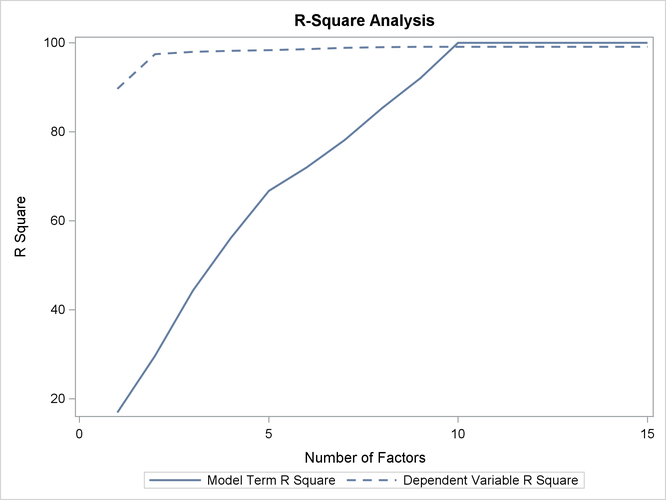
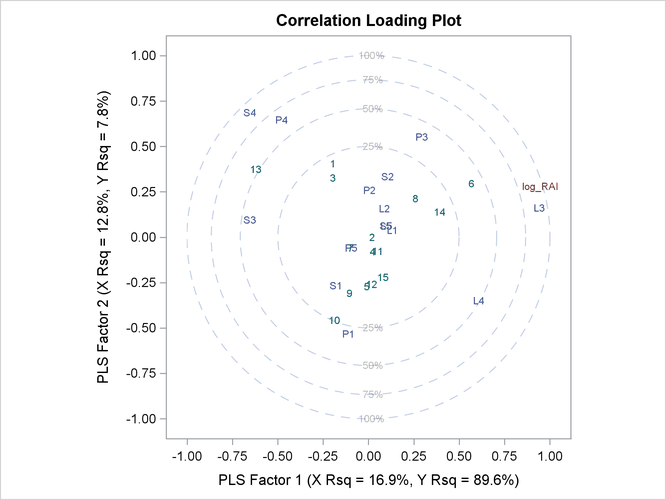
Output 70.1.2: Plot of Proportion of Variation Accounted For

Output 70.1.3: Correlation Loadings Plot

The plot in Output 70.1.2 of the proportion of variation explained (or R square) makes it clear that there is a plateau in the response variation after two factors are included in the model. The correlation loading plot in Output 70.1.3 summarizes many features of this two-factor model, including the following:

The X-scores are plotted as numbers for each observation. You should look for patterns or clearly grouped observations. If you see a curved pattern, for example, you might want to add a quadratic term. Two or more groupings of observations indicate that it might be better to analyze the groups separately, perhaps by including classification effects in the model. This plot appears to show most of the observations close together, with a few being more spread out with larger positive X-scores for factor 2. There are no clear grouping patterns, but observation 13 stands out.
The loadings show how much variation in each variable is accounted for by the first two factors, jointly by the distance of the corresponding point from the origin and individually by the distance for the projections of this point onto the horizontal and vertical axes. That the dependent variable is well explained by the model is reflected in the fact that the point for log_RAI is near the 100% circle.
You can also use the projection interpretation to relate variables to each other. For example, projecting other variables’ points onto the line that runs through the log_RAI point and the origin, you can see that the PLS approximation for the predictor L3 is highly positively correlated with log_RAI, S3 is somewhat less correlated but in the negative direction, and several predictors including L1, L5, and S5 have very little correlation with log_RAI.

Other graphics enable you to explore more of the features of the PLS model. For example, you can examine the X-scores versus the Y-scores to explore how partial least squares chooses successive factors. For a good PLS model, the first few factors show a high correlation between the X- and Y-scores. The correlation usually decreases from one factor to the next. When ODS Graphics is enabled, you can plot the X-scores versus the Y-scores by using the PLOT=XYSCORES option, as shown in the following statements.

proc pls data=pentaTrain nfac=4 plot=XYScores;
   model log_RAI = S1-S5 L1-L5 P1-P5;
run;

The plot of the X-scores versus the Y-scores for the first four factors is shown in Output 70.1.4.

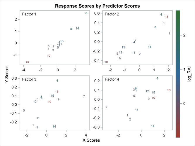
Output 70.1.4: X-Scores versus Y-Scores

For this example, Output 70.1.4 shows high correlation between X- and Y-scores for the first factor but somewhat lower correlation for the second factor and sharply diminishing correlation after that. This adds strength to the judgment that NFAC=2 is the right number of factors for these data and this model. Note that observation 13 is again extreme in the first two plots. This run might be overly influential for the PLS analysis; thus, you should check to make sure it is reliable.

As explained earlier, you can draw some inferences about the relationship between individual predictors and the dependent variable from the correlation loading plot. However, the regression coefficient profile and the variable importance plot give a more direct indication of which predictors are most useful for predicting the dependent variable. The regression coefficients represent the importance each predictor has in the prediction of just the response. The variable importance plot, on the other hand, represents the contribution of each predictor in fitting the PLS model for both predictors and response. It is based on the Variable Importance for Projection (VIP) statistic of Wold (1994), which summarizes the contribution a variable makes to the model. If a predictor has a relatively small coefficient (in absolute value) and a small value of VIP, then it is a prime candidate for deletion. Wold in Umetrics (1995) considers a value less than 0.8 to be “small” for the VIP. The following statements fit a two-factor PLS model and display these two additional plots.

proc pls data=pentaTrain nfac=2 plot=(ParmProfiles VIP);
   model log_RAI = S1-S5 L1-L5 P1-P5;
run;

ods graphics off;

The additional graphics are shown in Output 70.1.5 and Output 70.1.6.

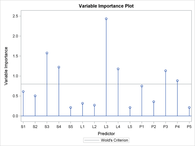
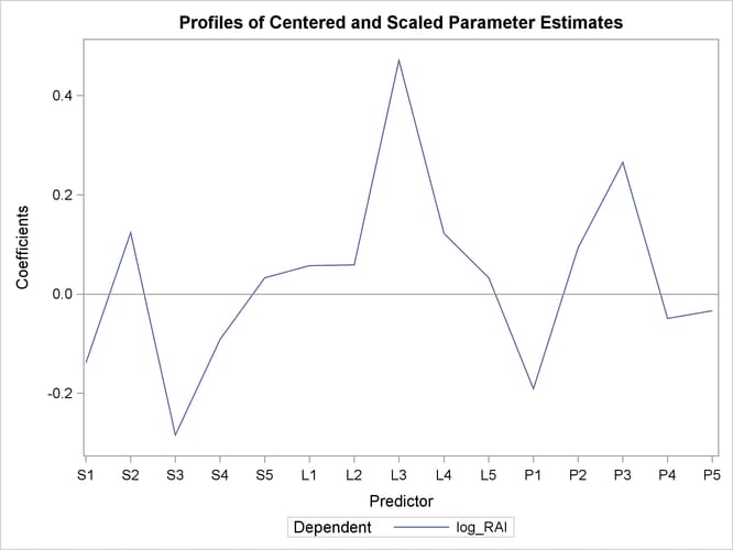
Output 70.1.5: Variable Importance Plots

Output 70.1.6: Regression Parameter Profile

In these two plots, the variables L1, L2, P2, S5, L5, and P5 have small absolute coefficients and small VIP. Looking back at the correlation loadings plot in Output 70.1.2, you can see that these variables tend to be the ones near zero for both PLS factors. You should consider dropping these variables from the model.