The ORTHOREG Procedure

The extra accuracy of the regression algorithm used by PROC ORTHOREG is most useful when the model contains near-singularities that you want to be able to distinguish from true singularities. This example demonstrates this usefulness in the context of fitting polynomials of high degree.
Note: The results from this example vary from machine to machine, depending on floating-point configuration.
The following DATA step computes a response y as an exact ninth-degree polynomial function of a predictor x evaluated at 0, 0.01, 0.02, …, 1.
title 'Polynomial Data';
data Polynomial;
   do i = 1 to 101;
      x = (i-1)/(101-1);
      y = 10**(9/2);
      do j = 0 to 8;
         y = y * (x - j/8);
      end;
      output;
   end;
run;
The polynomial is constructed in such a way that its zeros lie at ![]() for
for ![]() . The following statements use the EFFECT statement to fit a ninth-degree polynomial to this data with PROC ORTHOREG. The
EFFECT statement makes it easy to specify complicated polynomial models.
. The following statements use the EFFECT statement to fit a ninth-degree polynomial to this data with PROC ORTHOREG. The
EFFECT statement makes it easy to specify complicated polynomial models.
ods graphics on;

proc orthoreg data=Polynomial;
   effect xMod = polynomial(x / degree=9);
   model y = xMod;
   effectplot fit / obs;
   store OStore;
run;

ods graphics off;
The effect xMod defined by the EFFECT statement refers to all nine degrees of freedom in the ninth-degree polynomial (excluding the intercept
term). The resulting output is shown in Output 66.3.1. Note that the R square for the fit is 1, indicating that the ninth-degree polynomial has been correctly fit.
Output 66.3.1: PROC ORTHOREG Results for Ninth-Degree Polynomial
| Polynomial Data |
| Source | DF | Sum of Squares | Mean Square | F Value | Pr > F |
|---|---|---|---|---|---|
| Model | 9 | 15.527180055 | 1.7252422284 | 1.65E22 | <.0001 |
| Error | 91 | 9.496616E-21 | 1.043584E-22 | ||
| Corrected Total | 100 | 15.527180055 |
| Root MSE | 1.02156E-11 |
|---|---|
| R-Square | 1 |
| Parameter | DF | Parameter Estimate | Standard Error | t Value | Pr > |t| |
|---|---|---|---|---|---|
| Intercept | 1 | -3.24572035915E-11 | 8.114115E-12 | -4.00 | 0.0001 |
| x | 1 | 75.9977312440678 | 4.898326E-10 | 1.55E11 | <.0001 |
| x^2 | 1 | -1652.40781362191 | 9.5027919E-9 | -174E9 | <.0001 |
| x^3 | 1 | 14249.4539769783 | 8.3110512E-8 | 1.71E11 | <.0001 |
| x^4 | 1 | -64932.461575205 | 3.8997072E-7 | -167E9 | <.0001 |
| x^5 | 1 | 173315.359360779 | 1.066611E-6 | 1.62E11 | <.0001 |
| x^6 | 1 | -280158.03646002 | 1.7523078E-6 | -16E10 | <.0001 |
| x^7 | 1 | 269781.812887653 | 1.7021134E-6 | 1.58E11 | <.0001 |
| x^8 | 1 | -142302.494710055 | 9.0027891E-7 | -158E9 | <.0001 |
| x^9 | 1 | 31622.7766022468 | 1.997493E-7 | 1.58E11 | <.0001 |
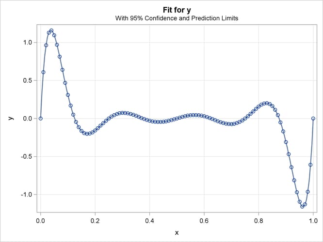
The fit plot produced by the EFFECTPLOT statement, Output 66.3.2, also demonstrates the perfect fit.
Finally, you can use the PLM procedure with the fit model saved by the STORE statement in the item store OStore to check the predicted values for the known zeros of the polynomial, as shown in the following statements:
data Zeros(keep=x);
   do j = 0 to 8;
      x = j/8;
      output;
   end;
run;

proc plm restore=OStore noprint;
   score data=Zeros out=OZeros pred=OPred;
run;

proc print noobs;
run;
The predicted values of the zeros, shown in Output 66.3.3, are again all miniscule.
Output 66.3.3: Predicted Zeros for Ninth-Degree Polynomial
| Polynomial Data |
| x | OPred |
|---|---|
| 0.000 | -3.2457E-11 |
| 0.125 | -2.1262E-11 |
| 0.250 | -9.5867E-12 |
| 0.375 | -2.2895E-11 |
| 0.500 | -5.2154E-11 |
| 0.625 | -1.2329E-10 |
| 0.750 | -2.5329E-10 |
| 0.875 | -3.9836E-10 |
| 1.000 | -5.9663E-10 |
To compare these results with those from a least squares fit produced by an alternative algorithm, consider fitting a polynomial to this data using the GLM procedure. PROC GLM does not have an EFFECT statement, but the familiar bar notation can still be used to specify a ninth-degree polynomial fairly succinctly, as shown in the following statements:
proc glm data=Polynomial;
   model y = x|x|x|x|x|x|x|x|x;
   store GStore;
run;
Partial results are shown in Output 66.3.4. In this case, the R square for the fit is only about 0.83, indicating that the full ninth-degree polynomial was not correctly fit.
Output 66.3.4: PROC GLM for Ninth-Degree Polynomial
| Polynomial Data |
| Source | DF | Sum of Squares | Mean Square | F Value | Pr > F |
|---|---|---|---|---|---|
| Model | 8 | 12.91166643 | 1.61395830 | 56.77 | <.0001 |
| Error | 92 | 2.61551363 | 0.02842950 | ||
| Corrected Total | 100 | 15.52718006 |
| R-Square | Coeff Var | Root MSE | y Mean |
|---|---|---|---|
| 0.831553 | -6.6691E17 | 0.168610 | -0.000000 |
The following statements, which use the PLM procedure to compute predictions based on the GLM fit at the true zeros of the polynomial, also confirm that PROC GLM is not able to correctly fit a polynomial of this degree, as shown in Output 66.3.5.
proc plm restore=GStore noprint;
   score data=Zeros out=GZeros pred=GPred;
run;

data Zeros;
   merge OZeros GZeros;
run;

proc print noobs;
run;
Output 66.3.5: Predicted Zeros for Ninth-Degree Polynomial
| Polynomial Data |
| x | OPred | GPred |
|---|---|---|
| 0.000 | -3.2457E-11 | 0.44896 |
| 0.125 | -2.1262E-11 | 0.22087 |
| 0.250 | -9.5867E-12 | -0.19037 |
| 0.375 | -2.2895E-11 | 0.12710 |
| 0.500 | -5.2154E-11 | 0.00000 |
| 0.625 | -1.2329E-10 | -0.12710 |
| 0.750 | -2.5329E-10 | 0.19037 |
| 0.875 | -3.9836E-10 | -0.22087 |
| 1.000 | -5.9663E-10 | -0.44896 |