The MULTTEST Procedure

Suppose you conduct a small study to test the effect of a drug on 15 subjects. You randomly divide the subjects into three balanced groups receiving 0 mg, 1 mg, and 2 mg of the drug, respectively. You carry out the experiment and record the presence or absence of 10 side effects for each subject. Your data set is as follows:
data Drug;
   input Dose$ SideEff1-SideEff10;
   datalines;
0MG  0   0   1   0   0   1   0   0   0   0
0MG  0   0   0   0   0   0   0   0   0   1
0MG  0   0   0   0   0   0   0   0   1   0
0MG  0   0   0   0   0   0   0   0   0   0
0MG  0   1   0   0   0   0   0   0   0   0
1MG  1   0   0   1   0   1   0   0   1   0
1MG  0   0   0   1   1   0   0   1   0   1
1MG  0   1   0   0   0   0   1   0   0   0
1MG  0   0   1   0   0   0   0   0   0   1
1MG  1   0   1   0   0   0   0   1   0   0
2MG  0   1   1   1   0   1   1   1   0   1
2MG  1   1   1   1   1   1   0   1   1   0
2MG  1   0   0   1   0   1   1   0   1   0
2MG  0   1   1   1   1   0   1   1   1   1
2MG  1   0   1   0   1   1   1   0   0   1
;
The increasing incidence of 1s for higher dosages in the preceding data set provides an initial visual indication that the drug has an effect. To explore this statistically, you perform an analysis in which the possibility of side effects increases linearly with drug level. You can analyze the data for each side effect separately, but you are concerned that, with so many tests, there might be a high probability of incorrectly declaring some drug effects significant. You want to correct for this multiplicity problem in a way that accounts for the discreteness of the data and for the correlations between observations on the same unit.
PROC MULTTEST addresses these concerns by processing all of the data simultaneously and adjusting the p-values. The following statements perform a typical analysis:
ods graphics on;
proc multtest bootstrap nsample=20000 seed=41287 notables
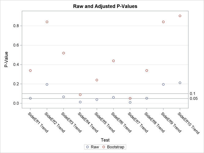
plots=PByTest(vref=0.05 0.1);
class Dose;
test ca(SideEff1-SideEff10);
contrast 'Trend' 0 1 2;
run;
ods graphics off;
This analysis uses the BOOTSTRAP option to adjust the p-values. The NSAMPLE= option requests 20,000 samples for the bootstrap analysis, and the starting seed for the random number generator is 41287. The NOTABLES option suppresses the display of summary statistics for each side effect and drug level combination. The PLOTS= option displays a visual summary of the unadjusted and adjusted p-values against each test, and the VREF= option adds reference lines to the display.
The CLASS statement is used to specify the grouping variable, Dose. The ca(sideeff1-sideeff10) specification in the TEST statement requests a Cochran-Armitage linear trend test for all 10 characteristics. The CONTRAST statement gives the coefficients for the linear trend test.
The “Model Information” table in Figure 61.1 describes the statistical tests performed by PROC MULTTEST. For this example, PROC MULTTEST carries out a two-tailed Cochran-Armitage linear trend test with no continuity correction or strata adjustment. This test is performed on the raw data and on 20,000 bootstrap samples.
Figure 61.1: Output Summary for the MULTTEST Procedure
| Model Information | |
|---|---|
| Test for discrete variables | Cochran-Armitage |
| Z-score approximation used | Everywhere |
| Continuity correction | 0 |
| Tails for discrete tests | Two-tailed |
| Strata weights | None |
| P-value adjustment | Bootstrap |
| Number of resamples | 20000 |
| Seed | 41287 |
The “Contrast Coefficients” table in Figure 61.2 displays the coefficients for the Cochran-Armitage test. They are 0, 1, and 2, as specified in the CONTRAST statement.
Figure 61.2: Coefficients Used in the MULTTEST Procedure
| Contrast Coefficients | |||
|---|---|---|---|
| Contrast | Dose | ||
| 0MG | 1MG | 2MG | |
| Trend | 0 | 1 | 2 |
The “p-Values” table in Figure 61.3 lists the p-values for the drug example. The Raw column lists the p-values for the Cochran-Armitage test on the original data, and the Bootstrap column provides the bootstrap adjustment of the raw p-values.
Note that the raw p-values lead you to reject the null hypothesis of no linear trend for 3 of the 10 characteristics at the 5% level and 7 of the 10 characteristics at the 10% level. The bootstrap p-values, however, lead to this conclusion for 0 of the 10 characteristics at the 5% level and only 2 of the 10 characteristics at the 10% level; you can also see this in Figure 61.4.
Figure 61.3: Summary of p-Values for the MULTTEST Procedure
| p-Values | |||
|---|---|---|---|
| Variable | Contrast | Raw | Bootstrap |
| SideEff1 | Trend | 0.0519 | 0.3388 |
| SideEff2 | Trend | 0.1949 | 0.8403 |
| SideEff3 | Trend | 0.0662 | 0.5190 |
| SideEff4 | Trend | 0.0126 | 0.0884 |
| SideEff5 | Trend | 0.0382 | 0.2408 |
| SideEff6 | Trend | 0.0614 | 0.4383 |
| SideEff7 | Trend | 0.0095 | 0.0514 |
| SideEff8 | Trend | 0.0519 | 0.3388 |
| SideEff9 | Trend | 0.1949 | 0.8403 |
| SideEff10 | Trend | 0.2123 | 0.9030 |
The bootstrap adjustment gives the probability of observing a p-value as extreme as each given p-value, considering all 10 tests simultaneously. This adjustment incorporates the correlation of the raw p-values, the discreteness of the data, and the multiple testing problem. Failure to account for these issues can certainly lead to misleading inferences for these data.