The LIFETEST Procedure
The data in this example come from Lee (1992, p. 91) and represent the survival rates of males with angina pectoris. Survival time is measured as years from the time
of diagnosis. In the following DATA step, the data are read as number of events and number of withdrawals in each one-year
time interval for 16 intervals. Three variables are constructed from the data: Years (an artificial time variable with values that are the midpoints of the time intervals), Censored (a censoring indicator variable with the value 1 indicating censored observations and the value 0 indicating event observations),
and Freq (the frequency variable). Two observations are created for each interval, one representing the event observations and the
other representing the censored observations.
title 'Survival of Males with Angina Pectoris';
data Males;
   keep Freq Years Censored;
   retain Years -.5;
   input fail withdraw @@;
   Years + 1;
   Censored=0;
   Freq=fail;
   output;
   Censored=1;
   Freq=withdraw;
   output;
   datalines;
456   0 226  39 152  22 171  23 135 24 125 107
 83 133  74 102  51  68  42  64  43 45  34  53
 18  33   9  27   6  23   0  30
;
In the following statements, the ODS GRAPHICS ON specification enables ODS Graphics. PROC LIFETEST is invoked to compute the various life-table survival estimates, the median residual time, and their standard errors. The life-table method of computing estimates is requested by specifying METHOD=LT. The intervals are specified by the INTERVAL= option. Graphical displays of the life-table survivor function estimate, negative log of the estimate, log of negative log of the estimate, estimated density function, and estimated hazard function are requested by the PLOTS= option. No tests for homogeneity are carried out because the data are not stratified.
ods graphics on;
proc lifetest data=Males  method=lt intervals=(0 to 15 by 1)
              plots=(s,ls,lls,h,p);
   time Years*Censored(1);
   freq Freq;
run;
ods graphics off;
Results of the life-table estimation are shown in Output 52.3.1. The five-year survival rate is 0.5193 with a standard error of 0.0103. The estimated median residual lifetime, which is 5.33 years initially, reaches a maximum of 6.34 years at the beginning of the second year and decreases gradually to a value lower than the initial 5.33 years at the beginning of the seventh year.
Output 52.3.1: Life-Table Survivor Function Estimate
| Survival of Males with Angina Pectoris |
| Life Table Survival Estimates | |||||||||||||||
|---|---|---|---|---|---|---|---|---|---|---|---|---|---|---|---|
| Interval | Number Failed |
Number Censored |
Effective Sample Size |
Conditional Probability of Failure |
Conditional Probability Standard Error |
Survival | Failure | Survival Standard Error |
Median Residual Lifetime |
Median Standard Error |
Evaluated at the Midpoint of the Interval | ||||
| [Lower, | Upper) | PDF Standard Error |
Hazard | Hazard Standard Error |
|||||||||||
| 0 | 1 | 456 | 0 | 2418.0 | 0.1886 | 0.00796 | 1.0000 | 0 | 0 | 5.3313 | 0.1749 | 0.1886 | 0.00796 | 0.208219 | 0.009698 |
| 1 | 2 | 226 | 39 | 1942.5 | 0.1163 | 0.00728 | 0.8114 | 0.1886 | 0.00796 | 6.2499 | 0.2001 | 0.0944 | 0.00598 | 0.123531 | 0.008201 |
| 2 | 3 | 152 | 22 | 1686.0 | 0.0902 | 0.00698 | 0.7170 | 0.2830 | 0.00918 | 6.3432 | 0.2361 | 0.0646 | 0.00507 | 0.09441 | 0.007649 |
| 3 | 4 | 171 | 23 | 1511.5 | 0.1131 | 0.00815 | 0.6524 | 0.3476 | 0.00973 | 6.2262 | 0.2361 | 0.0738 | 0.00543 | 0.119916 | 0.009154 |
| 4 | 5 | 135 | 24 | 1317.0 | 0.1025 | 0.00836 | 0.5786 | 0.4214 | 0.0101 | 6.2185 | 0.1853 | 0.0593 | 0.00495 | 0.108043 | 0.009285 |
| 5 | 6 | 125 | 107 | 1116.5 | 0.1120 | 0.00944 | 0.5193 | 0.4807 | 0.0103 | 5.9077 | 0.1806 | 0.0581 | 0.00503 | 0.118596 | 0.010589 |
| 6 | 7 | 83 | 133 | 871.5 | 0.0952 | 0.00994 | 0.4611 | 0.5389 | 0.0104 | 5.5962 | 0.1855 | 0.0439 | 0.00469 | 0.1 | 0.010963 |
| 7 | 8 | 74 | 102 | 671.0 | 0.1103 | 0.0121 | 0.4172 | 0.5828 | 0.0105 | 5.1671 | 0.2713 | 0.0460 | 0.00518 | 0.116719 | 0.013545 |
| 8 | 9 | 51 | 68 | 512.0 | 0.0996 | 0.0132 | 0.3712 | 0.6288 | 0.0106 | 4.9421 | 0.2763 | 0.0370 | 0.00502 | 0.10483 | 0.014659 |
| 9 | 10 | 42 | 64 | 395.0 | 0.1063 | 0.0155 | 0.3342 | 0.6658 | 0.0107 | 4.8258 | 0.4141 | 0.0355 | 0.00531 | 0.112299 | 0.017301 |
| 10 | 11 | 43 | 45 | 298.5 | 0.1441 | 0.0203 | 0.2987 | 0.7013 | 0.0109 | 4.6888 | 0.4183 | 0.0430 | 0.00627 | 0.155235 | 0.023602 |
| 11 | 12 | 34 | 53 | 206.5 | 0.1646 | 0.0258 | 0.2557 | 0.7443 | 0.0111 | . | . | 0.0421 | 0.00685 | 0.17942 | 0.030646 |
| 12 | 13 | 18 | 33 | 129.5 | 0.1390 | 0.0304 | 0.2136 | 0.7864 | 0.0114 | . | . | 0.0297 | 0.00668 | 0.149378 | 0.03511 |
| 13 | 14 | 9 | 27 | 81.5 | 0.1104 | 0.0347 | 0.1839 | 0.8161 | 0.0118 | . | . | 0.0203 | 0.00651 | 0.116883 | 0.038894 |
| 14 | 15 | 6 | 23 | 47.5 | 0.1263 | 0.0482 | 0.1636 | 0.8364 | 0.0123 | . | . | 0.0207 | 0.00804 | 0.134831 | 0.054919 |
| 15 | . | 0 | 30 | 15.0 | 0 | 0 | 0.1429 | 0.8571 | 0.0133 | . | . | . | . | . | . |
The breakdown of event and censored observations in the data is shown in Output 52.3.2. Note that 32.8% of the patients have withdrawn from the study.
Output 52.3.2: Summary of Censored and Event Observations
| Summary of the Number of Censored and Uncensored Values |
|||
|---|---|---|---|
| Total | Failed | Censored | Percent Censored |
| 2418 | 1625 | 793 | 32.80 |
| Note: | 2 observations with invalid time, censoring, or frequency values were deleted. |
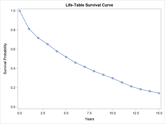
Output 52.3.3 displays the graph of the life-table survivor function estimate. The median survival time, read from the survivor function curve, is 5.33 years, and the 25th and 75th percentiles are 1.04 and 11.13 years, respectively.
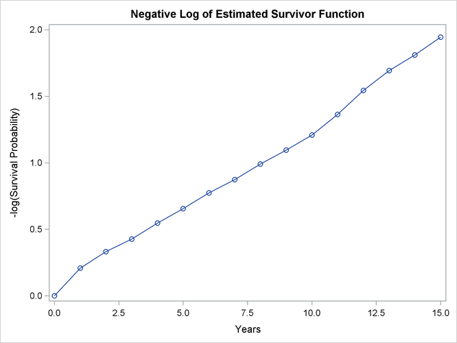
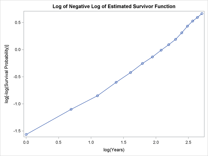
An exponential model might be appropriate for the survival of these male patients with angina pectoris since the curve of the negative log of the survivor function estimate versus the survival time (Output 52.3.4) approximates a straight line through the origin. Note that the graph of the log of the negative log of the survivor function estimate versus the log of time (Output 52.3.5) is practically a straight line.
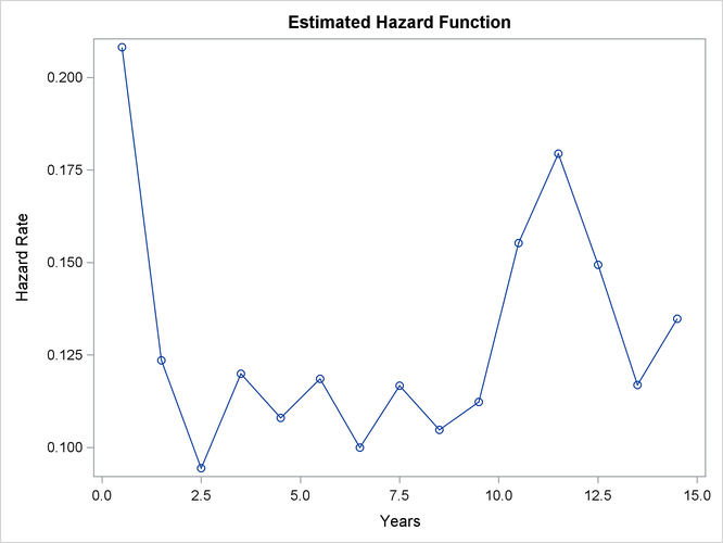
As discussed in Lee (1992), the graph of the estimated hazard function (Output 52.3.6) shows that the death rate is highest in the first year of diagnosis. From the end of the first year to the end of the tenth year, the death rate remains relatively constant, fluctuating between 0.09 and 0.12. The death rate is generally higher after the tenth year. This could indicate that a patient who has survived the first year has a better chance than a patient who has just been diagnosed. The profile of the median residual lifetimes also supports this interpretation.
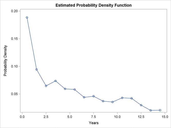
The density estimate is shown in (Output 52.3.7). Visually, it resembles the density function of an exponential distribution.

