The FMM Procedure

The FMM procedure calculates the log likelihood that corresponds to a particular response distribution according to the following formulas. The response distribution is the distribution specified (or chosen by default) through the DIST= option in the MODEL statement. The parameterizations used for log-likelihood functions of these distributions were chosen to facilitate expressions in terms of mean parameters that are modeled through an (inverse) link functions and in terms of scale parameters. These are not necessarily the parameterizations in which parameters of prior distributions are specified in a Bayesian analysis of homogeneous mixtures. See the section Prior Distributions for details about the parameterizations of prior distributions.
The FMM procedure includes all constant terms in the computation of densities or mass functions. In the expressions that follow,
l denotes the log-likelihood function, ![]() denotes a general scale parameter,
denotes a general scale parameter, ![]() is the “mean”, and
is the “mean”, and ![]() is a weight from the use of a WEIGHT statement.
is a weight from the use of a WEIGHT statement.
For some distributions (for example, the Weibull distribution) ![]() is not the mean of the distribution. The parameter
is not the mean of the distribution. The parameter ![]() is the quantity that is modeled as
is the quantity that is modeled as ![]() , where
, where ![]() is the inverse link function and the
is the inverse link function and the ![]() vector is constructed based on the effects in the MODEL statement. Situations in which the parameter
vector is constructed based on the effects in the MODEL statement. Situations in which the parameter ![]() does not represent the mean of the distribution are explicitly mentioned in the list that follows.
does not represent the mean of the distribution are explicitly mentioned in the list that follows.
The parameter ![]() is frequently labeled as a “Scale” parameter in output from the FMM procedure. It is not necessarily the scale parameter of the particular distribution.
is frequently labeled as a “Scale” parameter in output from the FMM procedure. It is not necessarily the scale parameter of the particular distribution.
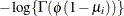
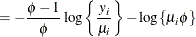
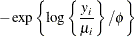
- Beta

-


This parameterization of the beta distribution is due to Ferrari and Cribari-Neto (2004) and has properties
![$\mr {E}[Y] = \mu $](images/statug_fmm0217.png) ,
, ![$\mr {Var}[Y] = \mu (1-\mu )/(1+\phi ), \, \phi > 0$](images/statug_fmm0218.png) .
.
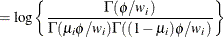
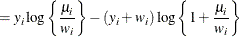
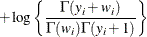
- Beta-binomial

-


where
 and
and  are the events and trials in the events/trials syntax and
  . This parameterization of the beta-binomial model presents the distribution as a special case of the Dirichlet-Multinomial
distribution—see, for example, Neerchal and Morel (1998). In this parameterization,
. This parameterization of the beta-binomial model presents the distribution as a special case of the Dirichlet-Multinomial
distribution—see, for example, Neerchal and Morel (1998). In this parameterization, ![$\mr {E}[Y] = n\mu $](images/statug_fmm0234.png) and
and ![$\mr {Var}[Y] = n\mu (1-\mu )(1+(n-1)/(\phi +1)), \, 0 \le \rho \le 1$](images/statug_fmm0235.png) . The FMM procedure models the parameter
. The FMM procedure models the parameter  and labels it “Scale” on the procedure output. For other parameterizations of the beta-binomial model, see Griffiths (1973) or Williams (1975).
- Binomial

-


where
and are the events and trials in the events/trials syntax and . In this parameterization , ![$\mr {Var}[Y] = n\mu (1-\mu )$](images/statug_fmm0243.png) .
.
- Binomial cluster

-


In this parameterization,
![$\mr {E}[Y] = n\pi $](images/statug_fmm0257.png) and
and ![$\mr {Var}[Y] = n\pi (1-\pi )\left\{ 1+\mu ^2(n-1)\right\} $](images/statug_fmm0258.png) . The binomial cluster model is a two-component mixture of a binomial
. The binomial cluster model is a two-component mixture of a binomial and a binomial
 random variable. This mixture is unusual in that it fixes the number of components and because the mixing probability
  appears in the moments of the mixture components. For further details, see Morel and Nagaraj (1993); Morel and Neerchal (1997); Neerchal and Morel (1998) and Example 37.1 in this chapter. The expressions for the mean and variance in the binomial cluster model are identical to those of the beta-binomial
model shown previously, with
appears in the moments of the mixture components. For further details, see Morel and Nagaraj (1993); Morel and Neerchal (1997); Neerchal and Morel (1998) and Example 37.1 in this chapter. The expressions for the mean and variance in the binomial cluster model are identical to those of the beta-binomial
model shown previously, with  ,
,  .
.
The FMM procedure models the parameter
 through the MODEL statement and the parameter through the PROBMODEL statement.
- Constant(c)
-
![\[ l(y_ i) = \left\{ \begin{array}{ll} 0 & y_ i = c \cr -1\mr {E}20 & y_ i \not= c \end{array}\right. \]](images/statug_fmm0263.png)
The extreme value when
 is chosen so that
  yields a likelihood of zero. You can change this value with the INVALIDLOGL= option in the PROC FMM statement. The constant distribution is useful for modeling overdispersion due to zero-inflation (or inflation of the process
at support c).
yields a likelihood of zero. You can change this value with the INVALIDLOGL= option in the PROC FMM statement. The constant distribution is useful for modeling overdispersion due to zero-inflation (or inflation of the process
at support c).
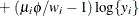
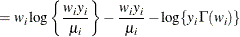
- Exponential

-
![\[ l(\mu _ i;y_ i,w_ i) = \left\{ \begin{array}{ll} -\log \{ \mu _ i\} - y_ i/\mu _ i & w_ i = 1 \cr w_ i\log \left\{ \frac{w_ iy_ i}{\mu _ i}\right\} - \frac{w_ iy_ i}{\mu _ i} - \log \{ y_ i \Gamma (w_ i)\} & w_ i \not= 1 \end{array} \right. \]](images/statug_fmm0267.png)
In this parameterization,
and ![$\mr {Var}[Y] = \mu ^2$](images/statug_fmm0268.png) .
.
- Folded normal

-


If X has a normal distribution with mean
and variance , then  has a folded normal distribution and log-likelihood function
  for
for  . The folded normal distribution arises, for example, when normally distributed measurements are observed, but their signs
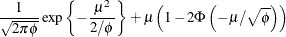
are not observed. The mean and variance of the folded normal in terms of the underlying
. The folded normal distribution arises, for example, when normally distributed measurements are observed, but their signs
are not observed. The mean and variance of the folded normal in terms of the underlying  distribution are
![$\displaystyle \mr {E}[Y] = $](images/statug_fmm0279.png)
![$\displaystyle \mr {Var}[Y] = $](images/statug_fmm0282.png)
![$\displaystyle \phi + \mu ^2 - \mr {E}[Y]^2 $](images/statug_fmm0283.png)
The FMM procedure models the folded normal distribution through the mean
and variance of the underlying normal distribution. When the FMM procedure computes output statistics for the response variable (for example
when you use the OUTPUT statement), the mean and variance of the response Y are reported. Similarly, the fit statistics apply to the distribution of , not the distribution of X. When you model a folded normal variable, the response input variable should be positive; the FMM procedure treats negative
values of Y as a support violation.
- Gamma
-
![\[ l(\mu _ i,\phi ;y_ i,w_ i) = w_ i\phi \log \left\{ \frac{w_ iy_ i\phi }{\mu _ i}\right\} - \frac{w_ iy_ i\phi }{\mu _ i} - \log \{ y_ i\} - \log \left\{ \Gamma (w_ i\phi )\right\} \]](images/statug_fmm0284.png)
In this parameterization,
and ![$\mr {Var}[Y] = \mu ^2/\phi , \, \phi > 0$](images/statug_fmm0285.png) . This parameterization of the gamma distribution differs from that in the GLIMMIX procedure, which expresses the log-likelihood
function in terms of
. This parameterization of the gamma distribution differs from that in the GLIMMIX procedure, which expresses the log-likelihood
function in terms of  in order to achieve a variance function suitable for mixed model analysis.
- Geometric
-

In this parameterization,
and ![$\mr {Var}[Y] = \mu + \mu ^2$](images/statug_fmm0291.png) . The geometric distribution is a special case of the negative binomial distribution with
. The geometric distribution is a special case of the negative binomial distribution with  .
.
- Generalized Poisson
-


In this parameterization,
![$\mr {E}[Y]=\mu $](images/statug_fmm0301.png) ,
, ![$\mr {Var}[Y] = \mu /(1-\xi )^2,$](images/statug_fmm0302.png) and
and  . The FMM procedure models the mean through the effects in the MODEL statement and applies a log link by default. The generalized Poisson distribution provides an overdispersed alternative to
the Poisson distribution;
. The FMM procedure models the mean through the effects in the MODEL statement and applies a log link by default. The generalized Poisson distribution provides an overdispersed alternative to
the Poisson distribution;  produces the mass function of a regular Poisson random variable. For details about the generalized Poisson distribution and
a comparison with the negative binomial distribution, see Joe and Zhu (2005).
produces the mass function of a regular Poisson random variable. For details about the generalized Poisson distribution and
a comparison with the negative binomial distribution, see Joe and Zhu (2005).
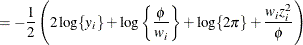
- Inverse Gaussian
-
![\[ l(\mu _ i,\phi ;y_ i,w_ i) = -\frac{1}{2} \left[ \frac{w_ i(y_ i-\mu _ i)^2}{y_ i\phi \mu _ i^2} + \log \left\{ \frac{\phi y_ i^3}{w_ i} \right\} + \log \{ 2\pi \} \right] \]](images/statug_fmm0305.png)
The variance is
![$\mr {Var}[Y] = \phi \mu ^3, \, \phi > 0$](images/statug_fmm0306.png) .
.
- Lognormal
-


If
 has a normal distribution with mean and variance , then Y has the log-likelihood function
  . The FMM procedure models the lognormal distribution and not the “shortcut” version you can obtain by taking the logarithm of a random variable and modeling that as normally distributed. The two approaches
are not equivalent, and the approach taken by PROC FMM is the actual lognormal distribution. Although the lognormal model
is a member of the exponential family of distributions, it is not in the “natural” exponential family because it cannot be written in canonical form.
. The FMM procedure models the lognormal distribution and not the “shortcut” version you can obtain by taking the logarithm of a random variable and modeling that as normally distributed. The two approaches
are not equivalent, and the approach taken by PROC FMM is the actual lognormal distribution. Although the lognormal model
is a member of the exponential family of distributions, it is not in the “natural” exponential family because it cannot be written in canonical form.
In terms of the parameters
and of the underlying normal process for X, the mean and variance of Y are ![$\mr {E}[Y] = \exp \{ \mu \} \sqrt {\omega }$](images/statug_fmm0314.png) and
and ![$\mr {Var}[Y] = \exp \{ 2\mu \} \omega (\omega -1)$](images/statug_fmm0315.png) , respectively, where
, respectively, where  . When you request predicted values with the OUTPUT statement, the FMM procedure computes
 ![$\mr {E}[Y]$](images/statug_fmm0317.png) and not .
and not .
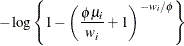
- Negative binomial
-
The variance is
![$\mr {Var}[Y] = \mu + \phi \mu ^2, \, \phi > 0$](images/statug_fmm0321.png) .
.
For a given
, the negative binomial distribution is a member of the exponential family. The parameter is related to the scale of the data because it is part of the variance function. However, it cannot be factored from the
variance, as is the case with the parameter in many other distributions.
- Normal
-
![\[ l(\mu _ i,\phi ;y_ i,w_ i) = -\frac{1}{2} \left[ \frac{w_ i(y_ i-\mu _ i)^2}{\phi } + \log \left\{ \frac{\phi }{w_ i}\right\} + \log \{ 2\pi \} \right] \]](images/statug_fmm0322.png)
The mean and variance are
and ![$\mr {Var}[Y] = \phi $](images/statug_fmm0323.png) , respectively,
, respectively, 
- Poisson
-
![\[ l(\mu _ i;y_ i,w_ i) = w_ i (y_ i \log \{ \mu _ i\} - \mu _ i - \log \{ \Gamma (y_ i + 1)\} ) \]](images/statug_fmm0324.png)
The mean and variance are
and ![$\mr {Var}[Y] = \mu $](images/statug_fmm0325.png) .
.
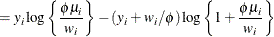
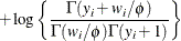
- (Shifted) T

-


In this parameterization
and ![$\mr {Var}[Y] = \phi \nu /(\nu -2), \, \phi > 0, \nu > 0$](images/statug_fmm0331.png) . Note that this form of the t distribution is not a non-central distribution, but that of a shifted central t random variable.
. Note that this form of the t distribution is not a non-central distribution, but that of a shifted central t random variable.
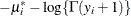
- Truncated Exponential

-

![$\displaystyle - \log \left[ \frac{\gamma \left(w_ i, \frac{w_ i b}{\mu _ i} \right)}{\Gamma (w_ i)} - \frac{\gamma \left(w_ i, \frac{w_ i a}{\mu _ i} \right)}{\Gamma (w_ i)} \right] $](images/statug_fmm0336.png)
where
![\[ \gamma (c_1, c_2) = \int _0^{c_2} t^{c_1-1} \exp (-t) \mr {d}t \]](images/statug_fmm0337.png)
is the lower incomplete gamma function. The mean and variance are
![$\displaystyle \mr {E}[Y] $](images/statug_fmm0338.png)
![$\displaystyle \mr {Var}[Y] $](images/statug_fmm0341.png)

![$\displaystyle - \left(\mr {E}[Y] \right)^2 $](images/statug_fmm0343.png)
- Truncated Lognormal

-

![$\displaystyle - \log \left\{ \Phi \left[ \sqrt {w_ i/\phi }(\log b - \mu _ i) \right] - \Phi \left[ \sqrt {w_ i/\phi }(\log a - \mu _ i) \right]\right\} $](images/statug_fmm0347.png)
where
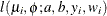
 is the cumulative distribution function of the standard normal distribution. The mean and variance are
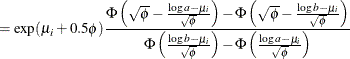
![$\displaystyle = \exp (2\mu _ i + 2\phi ) \frac{\Phi \left(2\sqrt {\phi } - \frac{\log a - \mu _ i}{\sqrt {\phi }} \right) - \Phi \left(2\sqrt {\phi } - \frac{\log b - \mu _ i}{\sqrt {\phi }} \right)}{\Phi \left(\frac{\log b - \mu _ i}{\sqrt {\phi }} \right) - \Phi \left(\frac{\log a - \mu _ i}{\sqrt {\phi }} \right)} - \left(\mr {E}[Y] \right)^2 $](images/statug_fmm0351.png)
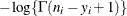
- Truncated Negative binomial
-

The mean and variance are
![$\displaystyle = (1 + \phi \mu _ i + \mu _ i) \mr {E}[Y] - \left(\mr {E}[Y] \right)^2 $](images/statug_fmm0357.png)
- Truncated Normal
-
![$\displaystyle = -\frac{1}{2} \left[ \frac{w_ i(y_ i-\mu _ i)^2}{\phi } + \log \left\{ \frac{\phi }{w_ i}\right\} + \log \{ 2\pi \} \right] $](images/statug_fmm0360.png)
![$\displaystyle - \log \left\{ \Phi \left[ \sqrt {w_ i/\phi }(b-\mu _ i) \right] - \Phi \left[ \sqrt {w_ i/\phi }(a-\mu _ i) \right]\right\} $](images/statug_fmm0361.png)
where
is the cumulative distribution function of the standard normal distribution. The mean and variance are
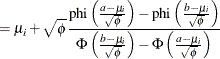
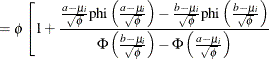
![$\displaystyle - \left. \left\{ \frac{\mr {phi}\left(\frac{a-\mu _ i}{\sqrt {\phi }} \right) - \mr {phi}\left(\frac{b-\mu _ i}{\sqrt {\phi }} \right)}{\Phi \left(\frac{b-\mu _ i}{\sqrt {\phi }} \right) - \Phi \left(\frac{a-\mu _ i}{\sqrt {\phi }} \right)}\right\} ^2 \right] $](images/statug_fmm0365.png)
where
 is the probability density function of the standard normal distribution.
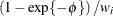
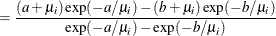
- Truncated Poisson
-
![\[ l(\mu _ i;y_ i,w_ i) = w_ i (y_ i \log \{ \mu _ i\} - \log \{ \exp (\mu _ i) - 1\} - \log \{ \Gamma (y_ i + 1)\} ) \]](images/statug_fmm0367.png)
The mean and variance are

![$\displaystyle = \frac{\mu _ i \left[1 - \exp (-\mu _ i) - \mu _ i \exp (-\mu _ i)\right]}{[1-\exp (-\mu _ i)]^2} $](images/statug_fmm0370.png)
- Uniform

-
![\[ l(\mu _ i;y_ i,w_ i) = -\log \{ b-a\} \]](images/statug_fmm0371.png)
The mean and variance are
![$\mr {E}[Y] = 0.5(a+b)$](images/statug_fmm0372.png) and
and ![$\mr {Var}[Y] = (b-a)^2/12$](images/statug_fmm0373.png) .
.
- Weibull
-

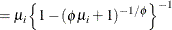
In this particular parameterization of the two-parameter Weibull distribution, the mean and variance of the random variable Y are
![$\mr {E}[Y] = \mu \Gamma (1+\phi )$](images/statug_fmm0378.png) and
and ![$\mr {Var}[Y] = \mu ^2\left\{ \Gamma (1+2\phi ) - \Gamma ^2(1+\phi ) \right\} $](images/statug_fmm0379.png) .
.