The VARIOGRAM Procedure

Computation of the Distribution Distance Classes
This section deals with theoretical considerations and practical aspects when you specify the LAGDISTANCE= and MAXLAGS= options. In principle, these values depend on the amount and spatial distribution of your experimental data.
The value of the LAGDISTANCE= option regulates how many pairs of data are contained within each distance class. In effect, this information defines the pairwise distance distribution (see the following subsection). Your choice of MAXLAGS= specifies how many of these lags you want to include in the empirical semivariogram computation. Adjusting the values of these parameters is a crucial part of your analysis. Based on your observations sample, they determine whether you have sufficient points for a descriptive empirical semivariogram, and they can affect the accuracy of the estimated semivariance, too.
The simplest way of determining the distribution of pairwise distances is to determine the maximum distance ![]() between any pair of points in your data, and then to divide this distance by some number N of intervals to produce distance classes of length
between any pair of points in your data, and then to divide this distance by some number N of intervals to produce distance classes of length ![]() . The distance
. The distance ![]() between each pair of points
between each pair of points ![]() is computed, and the pair
is computed, and the pair ![]() is counted in the kth distance class if
is counted in the kth distance class if ![]() for
for ![]() .
.
The actual computation is a slight variation of this. A bound, rather than the actual maximum distance, is computed. This
bound is the length of the diagonal of a bounding rectangle for the data points. This bounding rectangle is found by using
the maximum and minimum x and y coordinates, ![]() , and forming the rectangle determined by the following points:
, and forming the rectangle determined by the following points:
Table 102.5: (continued)
|
|
|
|
|
|
See Figure 102.24 for an illustration of the bounding rectangle applied to the data of the domain D in Figure 102.19. PROC VARIOGRAM provides you with the sizes of ![]() ,
, ![]() , and
, and ![]() . For example, in Figure 102.4 in the preliminary analysis, the specified parameters named “Max Data Distance in East,” “Max Data Distance in North,” and “Max Data Distance” correspond to the lengths
. For example, in Figure 102.4 in the preliminary analysis, the specified parameters named “Max Data Distance in East,” “Max Data Distance in North,” and “Max Data Distance” correspond to the lengths ![]() ,
, ![]() , and
, and ![]() , respectively.
, respectively.
Figure 102.24: Bounding Rectangle to Determine Maximum Pairwise Distance in Domain D
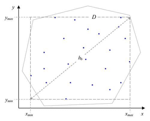
The pairwise distance bound, denoted by ![]() , is given by
, is given by
|
|
Using ![]() , the interval
, the interval ![]() is divided into
is divided into ![]() subintervals, where N is the value of the NHCLASSES= option specified in the COMPUTE statement, or N = 10 (default) if the NHCLASSES= option is not specified. The basic distance unit is
subintervals, where N is the value of the NHCLASSES= option specified in the COMPUTE statement, or N = 10 (default) if the NHCLASSES= option is not specified. The basic distance unit is ![]() ; the distance intervals are centered on
; the distance intervals are centered on ![]() , with a distance tolerance of
, with a distance tolerance of ![]() . The extra subinterval is
. The extra subinterval is ![]() and corresponds to lag class zero. It is half the length of the remaining subintervals, and it often contains the smallest
number of pairs. Figure 102.22 shows an example where the lag classes correspond to
and corresponds to lag class zero. It is half the length of the remaining subintervals, and it often contains the smallest
number of pairs. Figure 102.22 shows an example where the lag classes correspond to ![]() 1. This method of partitioning the interval
1. This method of partitioning the interval ![]() is used in the empirical semivariogram computation.
is used in the empirical semivariogram computation.
Choosing the Size of Classes
When you start with a data sample, the VARIOGRAM procedure computes all the distinct point pairs in the sample. The OUTPAIR= output data set, described in the section OUTPAIR=SAS-data-set, contains information about these pairs. The point pairs are then categorized in classes. The size of each class depends on the common distance that separates consecutive classes. In PROC VARIOGRAM you need to provide this distance value with the LAGDISTANCE= option. Practically, you can define the distance between classes to be about the size of the average sampling distance (Olea, 2006).
Under a more scrutinized approach, before you specify a value for the LAGDISTANCE= option, it is helpful to be aware of two issues. First, estimate how many classes of data pairs you might need. Each class contributes one point to the empirical semivariogram. Therefore, you need enough classes for an adequate number of points, so that your empirical semivariogram can suggest a suitable theoretical model shape for the description of the spatial continuity. Second, keep in mind that a larger number of data pairs in a class can contribute to a more accurate estimate of the corresponding semivariogram point.
The first consideration is a more general issue, and both this and the following subsection address it in detail. Based on the second consideration, the class size problem translates into having a sufficient number of data pairs in each class to produce an accurate semivariance estimate. However, only empirical rules of thumb exist to guide you with this choice. Examples of minimum-pairs empirical rules include the suggestion by Journel and Huijbregts (1978, p. 194) to use at least 30 point pairs for each lag class. Also, in a different approach, Chilès and Delfiner (1999, p. 38) increase this number to 50 point pairs.
Obviously, smaller data samples provide fewer data pairs in the sample. According to Olea (2006), it is difficult to properly estimate a semivariogram with fewer than 50 measurements. The preceding minimum-pairs practical rules are useful in cases where small samples are involved. When you work with a relatively small sample, the key is to specify the value of LAGDISTANCE= such that you can strike a balance between the number of the classes you can form and their pairs count. In the coal seam thickness example of the section Preliminary Spatial Data Analysis, it is not possible to create a desirable large number of classes and maintain an adequate size for each one. On the other hand, there is no practical need to invoke these rules in the case of the much larger sample of ozone concentrations in An Anisotropic Case Study with Surface Trend in the Data.
The spatial distribution of the sample might also affect the grouping of pairs into classes. For example, data that are sampled in clusters might prove difficult to classify according to the preceding practical rules. One strategy to address this problem is to accept fewer than 30 pairs for the underpopulated distance classes. Then, at the stage when you determine what theoretical semivariogram model to use, either disregard the corresponding empirical semivariogram points or use them and accept the increased uncertainty.
The VARIOGRAM procedure can help you decide on a suitable class size before you proceed with the empirical semivariogram computation. First, provide a number for the class count by specifying the NHCLASSES= value. Run the procedure with the option NOVARIOGRAM in the COMPUTE statement and examine the distribution data pairs. Use different values of NHCLASSES= to investigate how this parameter affects the data pairs distribution in each distance class. The pairwise distance intervals table (for example, Figure 102.3) shows the number of pairs in each distance class in the “Number of Pairs” column, and you can use the preceding rule of thumb to adjust the NHCLASSES= value accordingly.
PROC VARIOGRAM displays a rounded value of the distance between the lag bounds as the “Lag Distance” parameter in the pairs information table (see Figure 102.5) or the pairwise distances histogram (see Figure 102.4), which you can use for the LAGDISTANCE= specification. However, this is only one tool. For the semivariogram computation you can specify your own LAGDISTANCE= value based on your experience. Smaller LAGDISTANCE= values result in fewer data pairs in the classes. In that sense, you might find smaller values useful when you work with large samples so that you obtain more semivariogram points. Also, if the LAGDISTANCE= value is too large, you might end up “wasting” too many point pairs in fewer classes at the expense of computing fewer semivariogram points and no significant accuracy gains in the estimation.
As explained earlier, depending on the sample size and its spatial distribution you might have classes with fewer points than
what the practical rules advise. Most commonly, the deficient distance classes are the limiting ones close to the origin ![]() and the most remote ones at large
and the most remote ones at large ![]() . The classes near the origin correspond to lags 0 and 1. These lags are crucial because the empirical semivariogram in small
distances
. The classes near the origin correspond to lags 0 and 1. These lags are crucial because the empirical semivariogram in small
distances ![]() characterizes the process smoothness and can help you detect the presence of a nugget effect. However, as discussed in the
section Distance Classification, lag zero is half the size of the rest of the classes by definition, so it can be expected to violate the rule of thumb for
the number of pairs in a class.
characterizes the process smoothness and can help you detect the presence of a nugget effect. However, as discussed in the
section Distance Classification, lag zero is half the size of the rest of the classes by definition, so it can be expected to violate the rule of thumb for
the number of pairs in a class.
The classes located at higher and extreme distances within a spatial domain are often not accounted for in the empirical semivariogram. The fewer pairs that can be formed in these distances do not allow for an accurate assessment of the spatial correlation, as is explained in the following section.
Spatial Extent of the Empirical Semivariogram
Given your choice for the LAGDISTANCE= value in your spatial domain, the following paragraphs provide guidelines on how many classes to consider when you compute the empirical semivariogram.
Obviously, you want to include no more classes beyond the limit where the pairs count falls below the minimum-pairs empirical rule threshold, as discussed in the preceding subsection. PROC VARIOGRAM provides you with a visual way to inspect this upper limit, if you decide to make use of the minimum-pairs empirical rule. In particular, specify your threshold choice for the minimum pairs per class by using the THRESHOLD= parameter for the PLOTS=PAIRS option.
Then, the procedure produces in the pairwise distances histogram a reference line at the specified THRESHOLD= value, which leaves below the line all lags whose pairs count is lower than the threshold value; see, for example, Figure 102.4. The last lag class whose pair population is above the THRESHOLD= value is reported in the pairs information table as “Highest Lag With Pairs > Threshold.” This value is not a recommendation for the MAXLAGS= option, but rather is an upper limit for your choice. Detailed information about the pairs count in each class is displayed in the corresponding pairwise distance intervals table, as Figure 102.3 demonstrates.
The preceding suggests that you have an upper limit indication, but you still need some criterion to decide how many lags to include in the semivariogram estimation. The criterion is the extent of spatial dependence in your domain.
Spatial dependence can exist beyond your domain limits. However, you have no data past your domain scale to define a range for larger-scale spatial dependencies. As you look for pairs of data that are gradually farther apart, the number of pairs naturally decreases with distance. The pairs at the more distant classes might be so few that they are likely to be independent with respect to the spatial dependence scale that you can detect. If you include the largest distances in your empirical semivariogram plot, then these pairs only contribute added noise. In the same sense, you cannot explore in detail spatial dependencies in scales smaller than an average minimum distance between your data. The nugget effect represents then microscale correlations whose effect is evident in your working scale.
You specify the spatial dependence extent with commonly used measures such as the correlation range (or correlation length) ![]() and the correlation radius
and the correlation radius ![]() . Both are defined in a similar manner. The correlation range
. Both are defined in a similar manner. The correlation range ![]() is the distance at which the covariance is 5% of its value at
is the distance at which the covariance is 5% of its value at ![]() , and shows that beyond
, and shows that beyond ![]() the covariance is considered to be negligible. The correlation radius
the covariance is considered to be negligible. The correlation radius ![]() is the distance at which the covariance is about half the variance at
is the distance at which the covariance is about half the variance at ![]() , and indicates the distance over which significant correlations prevail (Christakos, 1992, p. 76). The physical meanings of these measures are similar to that of the semivariogram range. Also, the effective range
, and indicates the distance over which significant correlations prevail (Christakos, 1992, p. 76). The physical meanings of these measures are similar to that of the semivariogram range. Also, the effective range
![]() used in asymptotically increasing semivariance models has essentially the same definition as the correlation range
used in asymptotically increasing semivariance models has essentially the same definition as the correlation range ![]() (see the section Theoretical Semivariogram Models).
(see the section Theoretical Semivariogram Models).
A rough estimate of the correlation extent measures might be available from previous studies of a similar site, or from prior information about related measurements. In such an event, you typically want to consider a maximum pairwise distance that does not exceed the length of two or three correlation radii, or one and a half correlation ranges. You can then specify the MAXLAGS= value on the basis of the lags that fit in that distance.
When you have no estimates of correlation extent measures, you can use first use a crude measure to get started with your analysis: you can typically expect MAXLAGS= to be about half of the lag classes shown in the pairwise distances histogram.
Then, if necessary, you can refine your MAXLAGS= choice by using the following maximum lags rule of thumb: Journel and Huijbregts (1978, p. 194) advise considering lags up to about half of the extreme distance between data in the direction of interest. The
VARIOGRAM procedure assists you in this task by providing the overall extreme data distance ![]() , in addition to the extreme data distances in the vertical and horizontal axes directions. For example,
, in addition to the extreme data distances in the vertical and horizontal axes directions. For example, ![]() is reported in the pairs information table as “Maximum Data Distance” (see Figure 102.5), and in the pairwise distances histogram as “Max Data Distance” (see Figure 102.4).
is reported in the pairs information table as “Maximum Data Distance” (see Figure 102.5), and in the pairwise distances histogram as “Max Data Distance” (see Figure 102.4).
Overall, avoid significant deviations from the maximum lags rule of thumb. As was stated earlier, a MAXLAGS= value that takes you well beyond the half-extreme distance between data in a given direction might give you limited accuracy in the empirical semivariance estimates at higher distances. At the other end, a value of MAXLAGS= that is too small might lead you to omit important information about the spatial structure that potentially lies within the range of distances you skipped.