The MULTTEST Procedure

PROC MULTTEST Statement
PROC MULTTEST <options> ;
The PROC MULTTEST statement invokes the MULTTEST procedure. It also specifies the p-value adjustments. Table 61.1 summarizes the options available in the PROC MULTTEST statement. These options are described in alphabetical order following the table.
Table 61.1: PROC MULTTEST Statement Options by Function
|
Option |
Description |
|---|---|
|
FWE-Controlling p-Value Adjustments |
|
|
Computes the adaptive step-down Bonferroni adjustment |
|
|
Computes the adaptive step-up Bonferroni adjustment |
|
|
Computes the Bonferroni adjustment |
|
|
Computes the bootstrap min-p adjustment |
|
|
Computes Fisher’s combination adjustment |
|
|
Computes the step-up Bonferroni adjustment |
|
|
Computes Hommel’s adjustment |
|
|
Computes the step-down Bonferroni adjustment |
|
|
Computes the permutation min-p adjustment |
|
|
Computes Šidák’s adjustment |
|
|
Computes the step-down Bonferroni adjustment |
|
|
Computes the step-down bootstrap adjustment |
|
|
Computes the step-down permutation adjustment |
|
|
Computes the step-down Šidák adjustment |
|
|
Computes the Stouffer-Liptak combination adjustment |
|
|
FDR-Controlling p-Value Adjustments |
|
|
Computes the adaptive linear step-up adjustment |
|
|
Computes the linear step-up adjustment under dependence |
|
|
Computes the linear step-up adjustment |
|
|
Computes the linear step-up bootstrap min-p adjustment |
|
|
Computes the linear step-up permutation min-p adjustment |
|
|
Computes the positive FDR adjustment |
|
|
Input/Output Data Sets |
|
|
Names the input data set |
|
|
Names the input data set of raw p-values |
|
|
Names the output data set |
|
|
Names the output permutation data set |
|
|
Names the output resample data set |
|
|
Displayed Output Options |
|
|
Suppresses all tables |
|
|
Suppresses variable tables |
|
|
Suppresses zero tables for CLASS variables |
|
|
Suppresses the “p-Values” table |
|
|
Requests ODS Graphics |
|
|
Resampling Options |
|
|
Mean-centers continuous variables before resampling |
|
|
Does not mean-center continuous variables before resampling |
|
|
Specifies the number of resamples |
|
|
Specifies a different random number generator |
|
|
Specifies the seed for resampling |
|
|
CLASS Variable Options |
|
|
Suppresses zero tables for CLASS variables |
|
|
Specifies CLASS variable order |
|
|
Computational Options |
|
|
Specifies the comparison value |
|
|
Specifies the estimation method for the number of true nulls |
|
|
Specifies the estimation method for the proportion of true nulls |
|
You can specify the following options in the PROC MULTTEST statement.
-
ADAPTIVEHOCHBERG
AHOC -
requests adjusted p-values by using the Hochberg and Benjamini (1990) adaptive step-up Bonferroni method. See the section Adaptive Adjustments for more details.
-
ADAPTIVEHOLM
AHOLM -
requests adjusted p-values by using the Hochberg and Benjamini (1990) adaptive step-down Bonferroni method. See the section Adaptive Adjustments for more details.
-
ADAPTIVEFDR<(UNRESTRICT)>
AFDR<(UNRESTRICT)> -
requests adjusted p-values by using the Benjamini and Hochberg (2000) adaptive linear step-up method (AFDR). The UNRESTRICT option estimates the AFDR as defined in Benjamini and Hochberg (2000), which allows the adjustment to reduce the raw p-value. By default, the AFDR is constrained to be greater than or equal to the raw p-value. See the section Adaptive False Discovery Rate for more details.
-
BONFERRONI
BON -
specifies that the Bonferroni adjustments (number of tests
 p-value) be computed for each test. These adjustments can be extremely conservative and should be viewed with caution. When
exact tests are specified via the PERMUTATION= option in the TEST statement, the actual permutation distributions are used, resulting in a much less conservative version of this procedure
(Westfall and Wolfinger, 1997). See the section Bonferroni for more details.
p-value) be computed for each test. These adjustments can be extremely conservative and should be viewed with caution. When
exact tests are specified via the PERMUTATION= option in the TEST statement, the actual permutation distributions are used, resulting in a much less conservative version of this procedure
(Westfall and Wolfinger, 1997). See the section Bonferroni for more details.
-
BOOTSTRAP
BOOT -
specifies that the p-values be adjusted by using the bootstrap method to resample vectors (Westfall and Young, 1993). Resampling is performed with replacement and independently within levels of the STRATA variable. Continuous variables are mean-centered by default prior to resampling; specify the NOCENTER option to change this. See the section Bootstrap for more details. The BOOTSTRAP option is not allowed with the Peto test.
If the PERMUTATION= suboption is used with the CA test in the TEST statement, the exact permutation distribution is recomputed for each bootstrap sample. Caution: This can be very time-consuming. It is preferable to use permutation resampling when permutation base tests are used.
- CENTER
-
requests that continuous variables be mean-centered prior to resampling. The default action is to mean-center for bootstrap resampling and not to mean-center for permutation resampling.
- DATA=SAS-data-set
-
names the input SAS data set to be used by PROC MULTTEST. The default is to use the most recently created data set. The DATA= and INPVALUES= options cannot both be specified.
-
DEPENDENTFDR
DFDR -
requests adjusted p-values by using the method of Benjamini and Yekateuli (2001). See the section Dependent False Discovery Rate for more details.
- EPSILON=number
-
specifies the amount by which two p-values must differ to be declared unequal. The value number must be between 0 and 1; the default value is 1000 times the machine epsilon, which is approximately 1E–12. For SAS 9.1 and earlier releases the default value was 1E–8. See Westfall and Young (1993, pp. 165–166) for more information.
-
FDR
LSU -
requests adjusted p-values by using the linear step-up method of Benjamini and Hochberg (1995). These p-values do not control the familywise error rate, but they do control the false discovery rate in some cases. See the section False Discovery Rate Controlling Adjustments for more details.
-
FDRBOOT<(
 )>
)>
-
A bootstrap-resampling false discovery rate controlling method due to Yekateuli and Benjamini (1999). This method uses the same resampling algorithm as the BOOTSTRAP option. Every resample is saved in order to compute a quantile of the resampled p-values; therefore, this method can use a lot of memory. The parameter
 designates that a 100
 quantile is used in the computations for determining the adjustments; by default,
  . See the section False Discovery Rate Resampling Adjustments for details.
-
FDRPERM<(
)>
-
A permutation-resampling false discovery rate controlling method due to Yekateuli and Benjamini (1999). This method uses the same resampling algorithm as the PERMUTATION option. Every resample is saved in order to compute a quantile of the resampled p-values; therefore, this method can use a lot of memory. The parameter
designates that a 100 quantile is used in the computations for determining the adjustments; by default, . See the section False Discovery Rate Resampling Adjustments for details.
-
FISHER_C
FIC -
requests adjusted p-values by using Fisher’s combination method. See the section Fisher Combination for more details.
-
HOCHBERG
HOC -
requests adjusted p-values by using the step-up Bonferroni method due to Hochberg (1988). See the section Hochberg for more details.
-
HOMMEL
HOM -
requests adjusted p-values by using the method of Hommel (1988). See the section Hommel for more details.
- HOLM
-
is an alias for the STEPBON adjustment.
- INPVALUES<(pvalue-name)>=SAS-data-set
-
names an input SAS data set that includes a variable containing raw p-values. The MULTTEST procedure adjusts the collection of raw p-values for multiplicity. Resampling-based adjustments are not permitted with this type of data input. The CLASS, CONTRAST, FREQ, STRATA, and TEST statements are ignored when an INPVALUES= data set is specified. The INPVALUES= and DATA= options cannot both be specified. The pvalue-name enables you to specify the name of the p-value column from your data set. By default, pvalue-name=’raw_p’. The INPVALUES= data set can contain variables in addition to the raw p-values variable; see Example 61.5 for an example.
- LIPTAK
-
is an alias for the STOUFFER adjustment.
- NOCENTER
-
requests that continuous variables not be mean-centered prior to resampling. The default action is to mean-center for bootstrap resampling and not to mean-center for permutation resampling.
- NOPRINT
-
suppresses the normal display of results. Note that this option temporarily disables the Output Delivery System (ODS); see Chapter 20: Using the Output Delivery System, for more information.
- NOPVALUE
-
suppresses the display of the “p-Values” table of raw and adjusted p-values. This option is most useful when you are adjusting many tests and need to create only an OUT= data set or display graphics.
- NOTABLES
-
suppresses display of the “Discrete Variable Tabulations” and “Continuous Variable Tabulations” tables.
- NOZEROS
-
suppresses display of tables having zero occurrences for all CLASS levels.
-
NSAMPLE=number
N=number -
specifies the number of resamples for use with the resampling methods. The value number must be a positive integer; by default, 20,000 resamples are used. Large values of number (20,000 or more) are usually recommended for accuracy, but long execution times can result, particularly with large data sets.
-
NTRUENULL=keyword | value
M0=keyword | value -
Controls the method used to estimate the number of true NULL hypotheses (
 ) for the adaptive methods. This option is ignored unless one of the adaptive methods is specified. By default, PROC MULTTEST
uses the DECREASESLOPE method for the ADAPTIVEHOLM and ADAPTIVEHOCHBERG adjustments, and the LOWESTSLOPE method for ADAPTIVEFDR adjustment. For the PFDR adjustment, the SPLINE method is attempted first. If the estimate is nonpositive or if the slope of the spline at the last
) for the adaptive methods. This option is ignored unless one of the adaptive methods is specified. By default, PROC MULTTEST
uses the DECREASESLOPE method for the ADAPTIVEHOLM and ADAPTIVEHOCHBERG adjustments, and the LOWESTSLOPE method for ADAPTIVEFDR adjustment. For the PFDR adjustment, the SPLINE method is attempted first. If the estimate is nonpositive or if the slope of the spline at the last  is greater than 0.1 times the range of the fitted spline values, then the BOOTSTRAP method is used.
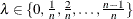
You can specify a positive integer as the value, or you can specify one of the keywords in the following list. Alternatively, you can specify the proportion of true NULL hypotheses by using the PTRUENULL= option. Suppose you have m tests with ordered p-values
 , and define
  .
.
- BOOTSTRAP<(bootstrap-options)>
-
uses the bootstrap method of Storey and Tibshirani (2003). Compute the proportion of true null hypotheses
 for
for  , where
  is the number of p-values less than or equal to , and f = 1 for the finite-sample case; otherwise f = 0. For each , bootstrap on the p-values to form B bootstrap versions
  , and choose the that yields the minimum
  . The available bootstrap-options are as follows:
- FINITE
-
the finite-sample case of the PFDR option.
- NBOOT=B
-
bootstrap resamples of the raw p-values for the
computations. NBOOT=10,000 by default; B must be a positive integer.
- NLAMBDA=n
-
“optimal”
is the value in  that minimizes the MSE. NLAMBD=20 by default; n must be an integer greater than 1.
- DECREASESLOPE
-
Schweder and Spjøtvoll (1982) as modified by Hochberg and Benjamini (1990). Let
 be the slope of the least squares line fit to
  and through the origin, for
  . Find the first
  such that
  . Then
  .
.
-
KSTEST<(
)>
-
uses the Kolmogorov-Smirnov uniformity test method of Turkheimer, Smith, and Schmidt (2001). Let
 , and the Kolmogorov-Smirnov statistic
  . If D is greater than the upper-tail probability (Press et al., 1992), then
  ; otherwise, let
  . Repeat until
  . Next compute the slope b of the weighted least squares regression line on the k smallest
  by using weights
  . Then
  .
.
- LEASTSQUARES
-
uses a linear least squares method to search for the correct cutpoint. For each
 compute the SSE of the least squares line through the origin fitting , let be the slope of this line, and add the SSE of the unconstrained least squares line through the rest of the qs. For i = 0 compute the SSE for the unconstrained line. The argument i that minimizes the SSE is the cutpoint: if i = 0 then
  ; if
; if  then
then  ; otherwise
 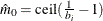 .
.
- LOWESTSLOPE
-
uses the lowest slope method of Benjamini and Hochberg (2000). Find the first
such that 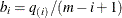 decreases. Then
 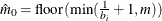 .
.
- MEANDIFF
-
uses the mean of differences method of Hsueh, Chen, and Kodell (2003). Let
 and estimate
  . Start from and proceed downward until the first time
  occurs.
- SPLINE<(spline-options)>
-
uses the cubic spline method of Storey and Tibshirani (2003). For each
 compute
 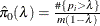 . Let
. Let  be the natural cubic spline with 3 degrees of freedom of
  versus . Estimate
  by taking the spline value at the last :
  , so that
  . The available spline-options are as follows:
- DF=df
-
sets the degrees of freedom of the spline, where df is a nonnegative integer. The default is DF=3.
- DFCONV=number
-
specifies the absolute change in spline degrees of freedom value for concluding convergence. If
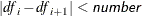 (or if the SPCONV= criterion is satisfied), then convergence is declared. number must be between 0 and 1; by default, number is 1000 times the square root of machine epsilon, which is about 1E–5.
- FINITE
-
computations for the finite-sample case of the PFDR option.
- MAXITER=n
-
specifies the maximum number of golden-search iterations used to find a spline with DF=
 degrees of freedom. By default, MAXITER=100; number must be a nonnegative integer.
- NLAMBDA=n
-
for for the spline fit. By default, NLAMBDA=20; number must be an integer greater than 1.
- SPCONV=number
-
specifies the absolute change in smoothing parameter value for concluding convergence of the spline. If
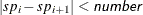 (or if the DFCONV= criterion is satisfied), then convergence is declared. By default, number equals the square root of the machine epsilon, which is about 1E–8.
In all cases
 is constrained to lie between 0 and m; if the computed
  , then the adaptive adjustments do not produce results. If you specify
  , then it is reduced to m. Values of are displayed in the “Estimated Number of True Null Hypotheses” table.
- ORDER=DATA | FORMATTED | FREQ | INTERNAL
-
specifies the sort order for the levels of the classification variables (which are specified in the CLASS statement). This option applies to the levels for all classification variables, except when you use the (default) ORDER=FORMATTED option with numeric classification variables that have no explicit format. With this option, the levels of such variables are ordered by their internal value.
The ORDER= option can take the following values:
Value of ORDER=
Levels Sorted By
DATA
Order of appearance in the input data set
FORMATTED
External formatted value, except for numeric variables with no explicit format, which are sorted by their unformatted (internal) value
FREQ
Descending frequency count; levels with the most observations come first in the order
INTERNAL
Unformatted value
By default, ORDER=FORMATTED. For ORDER=FORMATTED and ORDER=INTERNAL, the sort order is machine-dependent. For more information about sort order, see the chapter on the SORT procedure in the Base SAS Procedures Guide and the discussion of BY-group processing in SAS Language Reference: Concepts.
- OUT=SAS-data-set
-
names the output SAS data set containing variable names, contrast names, intermediate calculations, and all associated p-values. See OUT= Data Set for more information.
- OUTPERM=SAS-data-set
-
names the output SAS data set containing entire permutation distributions (upper-tail probabilities) for all tests when the PERMUTATION= option is specified. See OUTPERM= Data Set for more information. Caution: This data set can be very large.
- OUTSAMP=SAS-data-set
-
names the output SAS data set containing information from the resampled data sets when resampling is performed. See OUTSAMP= Data Set for more information. Caution: This data set can be very large.
- PDATA=SAS-data-set
-
is an alias for the INPVALUES= option.
-
PERMUTATION
PERM -
computes adjusted p-values in identical fashion as the BOOTSTRAP option, with the exception that PROC MULTTEST resamples without replacement rather than with replacement. Resampling is performed independently within levels of the STRATA variable. Continuous variables are not mean-centered prior to resampling; specify the CENTER to change this. See the section Bootstrap for more details. The PERMUTATION option is not allowed with the Peto test.
- PFDR<(options )>
-
computes the “q-values”
 of Storey (2002) and Storey, Taylor, and Siegmund (2004). PROC MULTTEST treats these “q-values” as adjusted p-values. The computations depend on selecting a parameter and an estimation method for the false discovery rate; see the section Positive False Discovery Rate for computational details. The available options for choosing the method are as follows:
- FINITE
-
estimates the false discovery rate with
 or
or  for the finite-sample case with independent null p-values.
- POSITIVE
-
estimates the false discovery rate with
instead of the default .
- UNRESTRICT
-
estimates the false discovery rate as defined in Storey (2002), which allows the adjustment to reduce the raw p-value. By default, the PFDR is constrained to be greater than or equal to the raw p-value.
The available options for controlling the
search are the bootstrap-options, the spline-options, and the following options:
- LAMBDA=number
-
specifies a
 and does not perform the bootstrap or spline searches for an “optimal” .
- MAXLAMBDA=number
-
stops the NLAMBDA= search sequence for the bootstrap and spline searches when this number is reached. The number must be in
![$[0,1]$](images/statug_multtest0058.png) . This option is ignored if the LAMBDA= option is specified.
. This option is ignored if the LAMBDA= option is specified.
-
PLOTS<(global-plot-options)>=plot-request<(options)>
PLOTS<(global-plot-options)>=(plot-request<(options)>< plot-request<(options)>> )
-
controls the plots produced through ODS Graphics. If you specify only one plot-request, you can omit the parentheses. For example, the following statements are valid specifications of the PLOTS= option:
plots = all
plots = (rawprob adjusted)
plots(sigonly) = (rawprob adjusted(unpack))
ODS Graphics must be enabled before plots can be requested. For example:
ods graphics on;
proc multtest plots=adjusted inpvalues=a pfdr;
run;
ods graphics off;
For more information about enabling and disabling ODS Graphics, see the section Enabling and Disabling ODS Graphics in Chapter 21: Statistical Graphics Using ODS.
By default, no graphs are created; you must specify the PLOTS= option to make graphs. You need at least two tests to produce a graph. If you are not using an INPVALUES= data set, then each test is given a name constructed as “variable-name contrast-label”. If you specify a MEAN test in the TEST statement, the t-test names are prefixed with “Mean:”. See Example 61.6 for examples of the ODS graphical displays.
The following global-plot-options are available:
- UNPACKPANELS | UNPACK
-
suppresses paneling. By default, the plots produced with the ADJUSTED and RAWPROB options are grouped in a single display, called a panel. Specify UNPACK to display each plot separately.
- SIGONLY<=number>
-
displays only those tests with adjusted p-values
 number, where
  number
  . By default, number = 0.05.
The following plot-requests are available:
- ADJUSTED<(UNPACK)>
-
displays a 2
2 panel of adjusted p-value plots similar to those Storey and Tibshirani (2003) developed for use with the PFDR p-value adjustment method. The plots of the adjusted p-values by the raw p-values and the adjusted p-values by their rank show the effect of the adjustments. The plot of the proportion of adjusted p-values each adjusted p-value and the plot of the expected number of false positives (the proportion significant multiplied by the adjusted p-value) versus the proportion significant show the effect of choosing different significance levels. The UNPACK option unpanels
the display.
- ALL
-
produces all appropriate plots. You can specify other options with ALL; for example, to display all plots and unpack the RAWPROB plots you can specify
plots=(all rawprob(unpack)). - LAMBDA
-
displays plots of the MSE and the estimated number of true nulls against the
parameter when the NTRUENULL=SPLINE or NTRUENULL=BOOTSTRAP option is in effect.
- MANHATTAN<(options)>
-
displays the Manhattan plot (a plot of –log
 of the adjusted p-values versus the tests). You can specify the following options:
- GROUP=variable
-
specifies a variable to group the adjusted p-values in the display.
- LABEL <=OBS>
-
labels the observations that have adjusted p-values that are less than the value specified in the VREF= option. By default, labels are created as follows: if an INPVALUES= data set and an ID statement are specified, then the observations are labeled with the ID values; if a DATA= data set is specified, then the observations are labeled with their constructed test name; otherwise, the observation or test number is displayed.
- NOTESTNAME
-
displays the number of the test instead of the test name on the X-axis, which is useful when you have many tests.
- UNPACK
-
suppresses paneling. By default, Manhattan plots are created for each requested p-value adjustment, and the results are grouped in a single display, called a panel. Specify UNPACK to display each plot separately.
- VREF=number | NONE
-
displays a reference line at –log
(number). The number must be between 0 and 1. By default, a reference line at –log(0.05) is displayed; it can be suppressed by specifying VREF=0 or VREF=NONE. If the LABEL option is also specified, then observations
above this line are labeled with their ID variables, their observation number, their test name, or their test number.
- NONE
-
suppresses all plots.
- PBYTEST<(options)>
-
displays the adjusted p-values for each test. The available options are as follows:
- RAWPROB<(UNPACK)>
-
displays a uniform probability plot of 1 minus the raw p-values (Schweder and Spjøtvoll, 1982) along with a histogram. If
is the number of true null hypotheses among the m tests, the points on the left side of the plot should be approximately linear with slope  . This graphic is displayed when an adaptive p-value adjustment method is requested in order to see if the NTRUENULL= estimate is appropriate. The UNPACK option unpanels the display.
-
PTRUENULL=keyword | value
PI0=keyword | value -
is alias for the NTRUENULL= option, except that you can specify the proportion of true null hypotheses as a value between 0 and 1, instead of specifying the number of true null hypotheses. The available keywords are also the NTRUENULL= options.
- RANUNI
-
requests the random number generator used in releases prior to SAS 9.2. Beginning with SAS 9.2, the random number generator is the Mersenne Twister, which has better performance when bootstrapping. Changes in the bootstrap- or permutation-adjusted p-values from prior releases are due to unimportant sampling differences.
-
SEED=number
S=number -
specifies the initial seed for the random number generator used for resampling. The value for number must be an integer. If you do not specify a seed, or if you specify a value less than or equal to zero, then PROC MULTTEST uses the time of day from the computer’s clock to generate an initial seed. For more details about seed values, see SAS Language Reference: Concepts.
-
SIDAK
SID -
computes the Šidák adjustment for each test. These adjustments take the form
![\[ 1 - (1 - p)^ m \]](images/statug_multtest0065.png)
where p is the raw p-value and m is the number of tests. These are slightly less conservative than the Bonferroni adjustments, but they still should be viewed with caution. When exact tests are specified via the PERMUTATION= option in the TEST statement, the actual permutation distributions are used, resulting in a much less conservative version of this procedure (Westfall and Wolfinger, 1997). See the section Šidák for more details.
-
STEPBON
HOLM -
requests adjusted p-values by using the step-down Bonferroni method of Holm (1979). See the section Step-Down Methods for more details.
- STEPBOOT
-
requests that adjusted p-values be computed by using bootstrap resampling as described under the BOOTSTRAP option, but in step-down fashion. See the section Step-Down Methods for more details.
- STEPPERM
-
requests that adjusted p-values be computed by using permutation resampling as described under the PERMUTATION option, but in step-down fashion. See the section Step-Down Methods for more details.
- STEPSID
-
requests adjusted p-values by using the Šidák method as described in the SIDAK option, but in step-down fashion. See the section Step-Down Methods for more details.
-
STOUFFER
LIPTAK -
requests adjusted p-values by using the Stouffer-Liptak combination method. See the section Stouffer-Liptak Combination for more details.