The LOGISTIC Procedure
- Overview
- Getting Started
-
Syntax
 PROC LOGISTIC StatementBY StatementCLASS StatementCODE StatementCONTRAST StatementEFFECT StatementEFFECTPLOT StatementESTIMATE StatementEXACT StatementEXACTOPTIONS StatementFREQ StatementID StatementLSMEANS StatementLSMESTIMATE StatementMODEL StatementNLOPTIONS StatementODDSRATIO StatementOUTPUT StatementROC StatementROCCONTRAST StatementSCORE StatementSLICE StatementSTORE StatementSTRATA StatementTEST StatementUNITS StatementWEIGHT Statement
 -
DetailsMissing ValuesResponse Level OrderingLink Functions and the Corresponding DistributionsDetermining Observations for Likelihood ContributionsIterative Algorithms for Model FittingConvergence CriteriaExistence of Maximum Likelihood EstimatesEffect-Selection MethodsModel Fitting InformationGeneralized Coefficient of DeterminationScore Statistics and TestsConfidence Intervals for ParametersOdds Ratio EstimationRank Correlation of Observed Responses and Predicted ProbabilitiesLinear Predictor, Predicted Probability, and Confidence LimitsClassification TableOverdispersionThe Hosmer-Lemeshow Goodness-of-Fit TestReceiver Operating Characteristic CurvesTesting Linear Hypotheses about the Regression CoefficientsRegression DiagnosticsScoring Data SetsConditional Logistic RegressionExact Conditional Logistic RegressionInput and Output Data SetsComputational ResourcesDisplayed OutputODS Table NamesODS Graphics
-
ExamplesStepwise Logistic Regression and Predicted ValuesLogistic Modeling with Categorical PredictorsOrdinal Logistic RegressionNominal Response Data: Generalized Logits ModelStratified SamplingLogistic Regression DiagnosticsROC Curve, Customized Odds Ratios, Goodness-of-Fit Statistics, R-Square, and Confidence LimitsComparing Receiver Operating Characteristic CurvesGoodness-of-Fit Tests and SubpopulationsOverdispersionConditional Logistic Regression for Matched Pairs DataFirth’s Penalized Likelihood Compared with Other ApproachesComplementary Log-Log Model for Infection RatesComplementary Log-Log Model for Interval-Censored Survival TimesScoring Data SetsUsing the LSMEANS StatementPartial Proportional Odds Model
- References
Example 54.14 Complementary Log-Log Model for Interval-Censored Survival Times
Often survival times are not observed more precisely than the interval (for instance, a day) within which the event occurred. Survival data of this form are known as grouped or interval-censored data. A discrete analog of the continuous proportional hazards model (Prentice and Gloeckler, 1978; Allison, 1982) is used to investigate the relationship between these survival times and a set of explanatory variables.
Suppose ![]() is the discrete survival time variable of the ith subject with covariates
is the discrete survival time variable of the ith subject with covariates ![]() . The discrete-time hazard rate
. The discrete-time hazard rate ![]() is defined as
is defined as
|
|
Using elementary properties of conditional probabilities, it can be shown that
|
|
Suppose ![]() is the observed survival time of the ith subject. Suppose
is the observed survival time of the ith subject. Suppose ![]() if
if ![]() is an event time and 0 otherwise. The likelihood for the grouped survival data is given by
is an event time and 0 otherwise. The likelihood for the grouped survival data is given by
|
|
|
|
|
|
|
|
|
|
|
|
where ![]() if the ith subject experienced an event at time
if the ith subject experienced an event at time ![]() and 0 otherwise.
and 0 otherwise.
Note that the likelihood L for the grouped survival data is the same as the likelihood of a binary response model with event probabilities ![]() . If the data are generated by a continuous-time proportional hazards model, Prentice and Gloeckler (1978) have shown that
. If the data are generated by a continuous-time proportional hazards model, Prentice and Gloeckler (1978) have shown that
|
|
which can be rewritten as
|
|
where the coefficient vector ![]() is identical to that of the continuous-time proportional hazards model, and
is identical to that of the continuous-time proportional hazards model, and ![]() is a constant related to the conditional survival probability in the interval defined by
is a constant related to the conditional survival probability in the interval defined by ![]() at
at ![]() . The grouped data survival model is therefore equivalent to the binary response model with complementary log-log link function.
To fit the grouped survival model by using PROC LOGISTIC, you must treat each discrete time unit for each subject as a separate
observation. For each of these observations, the response is dichotomous, corresponding to whether or not the subject died
in the time unit.
. The grouped data survival model is therefore equivalent to the binary response model with complementary log-log link function.
To fit the grouped survival model by using PROC LOGISTIC, you must treat each discrete time unit for each subject as a separate
observation. For each of these observations, the response is dichotomous, corresponding to whether or not the subject died
in the time unit.
Consider a study of the effect of insecticide on flour beetles. Four different concentrations of an insecticide were sprayed
on separate groups of flour beetles. The following DATA step saves the number of male and female flour beetles dying in successive
intervals in the data set Beetles:
data Beetles(keep=time sex conc freq);
   input time m20 f20 m32 f32 m50 f50 m80 f80;
   conc=.20; freq= m20; sex=1; output;
             freq= f20; sex=2; output;
   conc=.32; freq= m32; sex=1; output;
             freq= f32; sex=2; output;
   conc=.50; freq= m50; sex=1; output;
             freq= f50; sex=2; output;
   conc=.80; freq= m80; sex=1; output;
             freq= f80; sex=2; output;
   datalines;
 1   3   0  7  1  5  0  4  2
 2  11   2 10  5  8  4 10  7
 3  10   4 11 11 11  6  8 15
 4   7   8 16 10 15  6 14  9
 5   4   9  3  5  4  3  8  3
 6   3   3  2  1  2  1  2  4
 7   2   0  1  0  1  1  1  1
 8   1   0  0  1  1  4  0  1
 9   0   0  1  1  0  0  0  0
10   0   0  0  0  0  0  1  1
11   0   0  0  0  1  1  0  0
12   1   0  0  0  0  1  0  0
13   1   0  0  0  0  1  0  0
14 101 126 19 47  7 17  2  4
;
The data set Beetles contains four variables: time, sex, conc, and freq. The variable time represents the interval death time; for example, time=2 is the interval between day 1 and day 2. Insects surviving the duration (13 days) of the experiment are given a time value of 14. The variable sex represents the sex of the insects (1=male, 2=female), conc represents the concentration of the insecticide (mg/cm![]() ), and
), and freq represents the frequency of the observations.
To use PROC LOGISTIC with the grouped survival data, you must expand the data so that each beetle has a separate record for
each day of survival. A beetle that died in the third day (time=3) would contribute three observations to the analysis, one for each day it was alive at the beginning of the day. A beetle
that survives the 13-day duration of the experiment (time=14) would contribute 13 observations.
The following DATA step creates a new data set named Days containing the beetle-day observations from the data set Beetles. In addition to the variables sex, conc, and freq, the data set contains an outcome variable y and a classification variable day. The variable y has a value of 1 if the observation corresponds to the day that the beetle died, and it has a value of 0 otherwise. An observation
for the first day will have a value of 1 for day; an observation for the second day will have a value of 2 for day, and so on. For instance, Output 54.14.1 shows an observation in the Beetles data set with time=3, and Output 54.14.2 shows the corresponding beetle-day observations in the data set Days.
data Days;
   set Beetles;
   do day=1 to time;
      if (day < 14) then do;
         y= (day=time);
         output;
      end;
   end;
run;
Output 54.14.1: An Observation with Time=3 in Beetles Data Set
| Obs | time | conc | freq | sex |
|---|---|---|---|---|
| 17 | 3 | 0.2 | 10 | 1 |
Output 54.14.2: Corresponding Beetle-Day Observations in Days
| Obs | time | conc | freq | sex | day | y |
|---|---|---|---|---|---|---|
| 25 | 3 | 0.2 | 10 | 1 | 1 | 0 |
| 26 | 3 | 0.2 | 10 | 1 | 2 | 0 |
| 27 | 3 | 0.2 | 10 | 1 | 3 | 1 |
The following statements invoke PROC LOGISTIC to fit a complementary log-log model for binary data with the response variable
Y and the explanatory variables day, sex, and Variableconc. Specifying the EVENT= option ensures that the event (y=1) probability is modeled. The GLM coding in the CLASS statement creates an indicator column in the design matrix for each level of day. The coefficients of the indicator effects for day can be used to estimate the baseline survival function. The NOINT option is specified to prevent any redundancy in estimating the coefficients of day. The Newton-Raphson algorithm is used for the maximum likelihood estimation of the parameters.
proc logistic data=Days outest=est1;
   class day / param=glm;
   model y(event='1')= day sex conc
         / noint link=cloglog technique=newton;
   freq freq;
run;
Results of the model fit are given in Output 54.14.3. Both sex and conc are statistically significant for the survival of beetles sprayed by the insecticide. Female beetles are more resilient to
the chemical than male beetles, and increased concentration of the insecticide increases its effectiveness.
Output 54.14.3: Parameter Estimates for the Grouped Proportional Hazards Model
| Analysis of Maximum Likelihood Estimates | ||||||
|---|---|---|---|---|---|---|
| Parameter | DF | Estimate | Standard Error |
Wald Chi-Square |
Pr > ChiSq | |
| day | 1 | 1 | -3.9314 | 0.2934 | 179.5602 | <.0001 |
| day | 2 | 1 | -2.8751 | 0.2412 | 142.0596 | <.0001 |
| day | 3 | 1 | -2.3985 | 0.2299 | 108.8833 | <.0001 |
| day | 4 | 1 | -1.9953 | 0.2239 | 79.3960 | <.0001 |
| day | 5 | 1 | -2.4920 | 0.2515 | 98.1470 | <.0001 |
| day | 6 | 1 | -3.1060 | 0.3037 | 104.5799 | <.0001 |
| day | 7 | 1 | -3.9704 | 0.4230 | 88.1107 | <.0001 |
| day | 8 | 1 | -3.7917 | 0.4007 | 89.5233 | <.0001 |
| day | 9 | 1 | -5.1540 | 0.7316 | 49.6329 | <.0001 |
| day | 10 | 1 | -5.1350 | 0.7315 | 49.2805 | <.0001 |
| day | 11 | 1 | -5.1131 | 0.7313 | 48.8834 | <.0001 |
| day | 12 | 1 | -5.1029 | 0.7313 | 48.6920 | <.0001 |
| day | 13 | 1 | -5.0951 | 0.7313 | 48.5467 | <.0001 |
| sex | 1 | -0.5651 | 0.1141 | 24.5477 | <.0001 | |
| conc | 1 | 3.0918 | 0.2288 | 182.5665 | <.0001 | |
The coefficients of parameters for the day variable are the maximum likelihood estimates of ![]() , respectively. The baseline survivor function
, respectively. The baseline survivor function ![]() is estimated by
is estimated by
|
|
and the survivor function for a given covariate pattern (sex=![]() and
and conc=![]() ) is estimated by
) is estimated by
|
|
The following statements compute the survival curves for male and female flour beetles exposed to the insecticide in concentrations
of 0.20 mg/cm![]() and 0.80 mg/cm
and 0.80 mg/cm![]() :
:
data one (keep=day survival element s_m20 s_f20 s_m80 s_f80);
   array dd day1-day13;
   array sc[4] m20 f20 m80 f80;
   array s_sc[4] s_m20 s_f20 s_m80 s_f80 (1 1 1 1);
   set est1;
   m20= exp(sex + .20 * conc);
   f20= exp(2 * sex + .20 * conc);
   m80= exp(sex + .80 * conc);
   f80= exp(2 * sex + .80 * conc);
   survival=1;
   day=0;
   output;
   do over dd;
      element= exp(-exp(dd));
      survival= survival * element;
      do i=1 to 4;
         s_sc[i] = survival ** sc[i];
      end;
      day + 1;
      output;
   end;
run;
Instead of plotting the curves as step functions, the following statements use the PBSPLINE statement in the SGPLOT procedure to smooth the curves with a penalized B-spline. See Chapter 97: The TRANSREG Procedure, for details about the implementation of the penalized B-spline method. The SAS autocall macro %MODSTYLE is specified to change the marker symbols for the plot. For more information about the %MODSTYLE macro, see the section Style Template Modification Macro in Chapter 21: Statistical Graphics Using ODS. The smoothed survival curves are displayed in Output 54.14.4.
%modstyle(name=LogiStyle,parent=htmlblue,markers=circlefilled);
ods listing style=LogiStyle;
proc sgplot data=one;
   title 'Flour Beetles Sprayed with Insecticide';
   xaxis grid integer;
   yaxis grid label='Survival Function';
   pbspline y=s_m20 x=day /
      legendlabel = "Male at 0.20 conc." name="pred1";
   pbspline y=s_m80 x=day /
      legendlabel = "Male at 0.80 conc." name="pred2";
   pbspline y=s_f20 x=day /
      legendlabel = "Female at 0.20 conc." name="pred3";
   pbspline y=s_f80 x=day /
      legendlabel = "Female at 0.80 conc." name="pred4";
   discretelegend "pred1" "pred2" "pred3" "pred4" / across=2;
run;
Output 54.14.4: Predicted Survival at Insecticide Concentrations of 0.20 and 0.80 mg/cm![]()
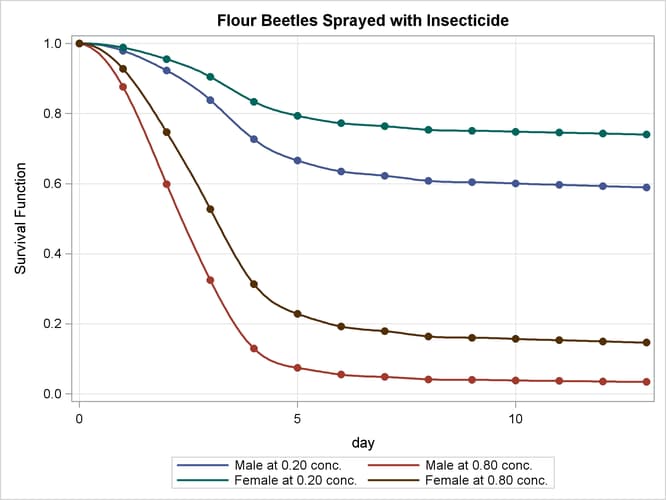
The probability of survival is displayed on the vertical axis. Notice that most of the insecticide effect occurs by day 6 for both the high and low concentrations.