The LIFETEST Procedure

Getting Started: LIFETEST Procedure
You can use the LIFETEST procedure to compute nonparametric estimates of the survivor functions, to compare survival curves, and to compute rank tests for association of the failure time variable with covariates.
For simple analyses, only the PROC LIFETEST and TIME statements are required. Consider a sample of survival data. Suppose
that the time variable is T and the censoring variable is C with value 1 indicating censored observations. The following statements compute the product-limit estimate for the sample:
proc lifetest;
   time t*c(1);
run;
You can use the STRATA statement to divide the data into various strata. A separate survivor function is then estimated for each stratum, and tests of the homogeneity of strata are performed. However, if the GROUP= option is also specified in the STRATA statement, the GROUP= variable is used to identify the samples whose survivor functions are to be compared, and the STRATA variables are used to define the strata for the stratified tests. You can specify covariates (prognostic variables) in the TEST statement, and PROC LIFETEST computes linear rank statistics to test the effects of these covariates on survival.
For example, consider the results of a small randomized trial on rats. Suppose you randomize 40 rats that have been exposed
to a carcinogen into two treatment groups (Drug X and Placebo). The event of interest is death from cancer induced by the carcinogen. The response is the time from randomization to death.
Four rats died of other causes; their survival times are regarded as censored observations. Interest lies in whether the survival
distributions differ between the two treatments.
The following DATA step creates the data set Exposed, which contains four variables: Days (survival time in days from treatment to death), Status (censoring indicator variable: 0 if censored and 1 if not censored), Treatment (treatment indicator), and Sex (gender: F if female and M if male).
proc format;
   value Rx 1='Drug X' 0='Placebo';
run;
data exposed;
   input Days  Status Treatment Sex $ @@;
   format Treatment Rx.;
   datalines;
179   1   1   F   378   0   1   M
256   1   1   F   355   1   1   M
262   1   1   M   319   1   1   M
256   1   1   F   256   1   1   M
255   1   1   M   171   1   1   F
224   0   1   F   325   1   1   M
225   1   1   F   325   1   1   M
287   1   1   M   217   1   1   F
319   1   1   M   255   1   1   F
264   1   1   M   256   1   1   F
237   0   0   F   291   1   0   M
156   1   0   F   323   1   0   M
270   1   0   M   253   1   0   M
257   1   0   M   206   1   0   F
242   1   0   M   206   1   0   F
157   1   0   F   237   1   0   M
249   1   0   M   211   1   0   F
180   1   0   F   229   1   0   F
226   1   0   F   234   1   0   F
268   0   0   M   209   1   0   F
;
PROC LIFETEST is invoked as follows to compute the product-limit estimate of the survivor function for each treatment and to compare the survivor functions between the two treatments:
ods graphics on;
proc lifetest data=Exposed plots=(survival(atrisk) logsurv);
   time Days*Status(0);
   strata Treatment;
run;
ods graphics off;
In the TIME statement, the survival time variable, Days, is crossed with the censoring variable, Status, with the value 0 indicating censoring. That is, the values of Days are considered censored if the corresponding values of Status are 0; otherwise, they are considered as event times. In the STRATA statement, the variable Treatment is specified, which indicates that the data are to be divided into strata based on the values of Treatment. ODS Graphics must be enabled before producing graphs. Two plots are requested through the PLOTS= option—a plot of the survival
curves with at risk numbers and a plot of the negative log of the survival curves.
The results of the analysis are displayed in the following figures.
Figure 52.1 displays the product-limit survival estimate for the Drug X group (Treatment=1). The figure lists, for each observed time, the survival estimate, failure rate, standard error of the estimate, cumulative
number of failures, and number of subjects remaining in the study.
Figure 52.1: Survivor Function Estimate for the Drug X-Treated Rats
| Product-Limit Survival Estimates | ||||||
|---|---|---|---|---|---|---|
| Days | Survival | Failure | Survival Standard Error |
Number Failed |
Number Left |
|
| 0.000 | 1.0000 | 0 | 0 | 0 | 20 | |
| 171.000 | 0.9500 | 0.0500 | 0.0487 | 1 | 19 | |
| 179.000 | 0.9000 | 0.1000 | 0.0671 | 2 | 18 | |
| 217.000 | 0.8500 | 0.1500 | 0.0798 | 3 | 17 | |
| 224.000 | * | . | . | . | 3 | 16 |
| 225.000 | 0.7969 | 0.2031 | 0.0908 | 4 | 15 | |
| 255.000 | . | . | . | 5 | 14 | |
| 255.000 | 0.6906 | 0.3094 | 0.1053 | 6 | 13 | |
| 256.000 | . | . | . | 7 | 12 | |
| 256.000 | . | . | . | 8 | 11 | |
| 256.000 | . | . | . | 9 | 10 | |
| 256.000 | 0.4781 | 0.5219 | 0.1146 | 10 | 9 | |
| 262.000 | 0.4250 | 0.5750 | 0.1135 | 11 | 8 | |
| 264.000 | 0.3719 | 0.6281 | 0.1111 | 12 | 7 | |
| 287.000 | 0.3187 | 0.6813 | 0.1071 | 13 | 6 | |
| 319.000 | . | . | . | 14 | 5 | |
| 319.000 | 0.2125 | 0.7875 | 0.0942 | 15 | 4 | |
| 325.000 | . | . | . | 16 | 3 | |
| 325.000 | 0.1062 | 0.8938 | 0.0710 | 17 | 2 | |
| 355.000 | 0.0531 | 0.9469 | 0.0517 | 18 | 1 | |
| 378.000 | * | 0.0531 | . | . | 18 | 0 |
| Note: | The marked survival times are censored observations. |
Figure 52.2 displays summary statistics of survival times for the Drug X group. It contains estimates of the 25th, 50th, and 75th percentiles and the corresponding 95% confidence limits. The median
survival time for rats in this treatment is 256 days. The mean and standard error are also displayed; however, these values
are underestimated because the largest observed time is censored and the estimation is restricted to the largest event time.
Figure 52.2: Summary Statistics of Survival Times for Drug X-Treated Rats
| Quartile Estimates | ||||
|---|---|---|---|---|
| Percent | Point Estimate |
95% Confidence Interval | ||
| Transform | [Lower | Upper) | ||
| 75 | 319.000 | LOGLOG | 256.000 | 355.000 |
| 50 | 256.000 | LOGLOG | 255.000 | 319.000 |
| 25 | 255.000 | LOGLOG | 171.000 | 256.000 |
| Mean | Standard Error |
|---|---|
| 271.131 | 11.877 |
| Note: | The mean survival time and its standard error were underestimated because the largest observation was censored and the estimation was restricted to the largest event time. |
Figure 52.3 and Figure 52.4 display the survival estimates and the summary statistics of the survival times for Placebo (Treatment=0). The median survival time for rats in this treatment is 235 days.
Figure 52.3: Survivor Function Estimate for Placebo-Treated Rats
| Product-Limit Survival Estimates | ||||||
|---|---|---|---|---|---|---|
| Days | Survival | Failure | Survival Standard Error |
Number Failed |
Number Left |
|
| 0.000 | 1.0000 | 0 | 0 | 0 | 20 | |
| 156.000 | 0.9500 | 0.0500 | 0.0487 | 1 | 19 | |
| 157.000 | 0.9000 | 0.1000 | 0.0671 | 2 | 18 | |
| 180.000 | 0.8500 | 0.1500 | 0.0798 | 3 | 17 | |
| 206.000 | . | . | . | 4 | 16 | |
| 206.000 | 0.7500 | 0.2500 | 0.0968 | 5 | 15 | |
| 209.000 | 0.7000 | 0.3000 | 0.1025 | 6 | 14 | |
| 211.000 | 0.6500 | 0.3500 | 0.1067 | 7 | 13 | |
| 226.000 | 0.6000 | 0.4000 | 0.1095 | 8 | 12 | |
| 229.000 | 0.5500 | 0.4500 | 0.1112 | 9 | 11 | |
| 234.000 | 0.5000 | 0.5000 | 0.1118 | 10 | 10 | |
| 237.000 | 0.4500 | 0.5500 | 0.1112 | 11 | 9 | |
| 237.000 | * | . | . | . | 11 | 8 |
| 242.000 | 0.3938 | 0.6063 | 0.1106 | 12 | 7 | |
| 249.000 | 0.3375 | 0.6625 | 0.1082 | 13 | 6 | |
| 253.000 | 0.2813 | 0.7188 | 0.1038 | 14 | 5 | |
| 257.000 | 0.2250 | 0.7750 | 0.0971 | 15 | 4 | |
| 268.000 | * | . | . | . | 15 | 3 |
| 270.000 | 0.1500 | 0.8500 | 0.0891 | 16 | 2 | |
| 291.000 | 0.0750 | 0.9250 | 0.0693 | 17 | 1 | |
| 323.000 | 0 | 1.0000 | . | 18 | 0 | |
| Note: | The marked survival times are censored observations. |
Figure 52.4: Summary Statistics of Survival Times for Placebo-Treated Rats
| Quartile Estimates | ||||
|---|---|---|---|---|
| Percent | Point Estimate |
95% Confidence Interval | ||
| Transform | [Lower | Upper) | ||
| 75 | 257.000 | LOGLOG | 237.000 | 323.000 |
| 50 | 235.500 | LOGLOG | 206.000 | 253.000 |
| 25 | 207.500 | LOGLOG | 156.000 | 229.000 |
| Mean | Standard Error |
|---|---|
| 235.156 | 10.211 |
A summary of the number of censored and event observations is shown in Figure 52.5. The figure lists, for each stratum, the number of event and censored observations, and the percentage of censored observations.
Figure 52.5: Number of Event and Censored Observations
| Summary of the Number of Censored and Uncensored Values | |||||
|---|---|---|---|---|---|
| Stratum | Treatment | Total | Failed | Censored | Percent Censored |
| 1 | Drug X | 20 | 18 | 2 | 10.00 |
| 2 | Placebo | 20 | 18 | 2 | 10.00 |
| Total | 40 | 36 | 4 | 10.00 | |
Figure 52.6 displays the graph of the product-limit survivor function estimates versus survival time. The two treatments differ primarily at larger survival times. Note the number of subjects at risk in the plot. You can display the number of subjects at risk at specific time points by using the ATRISK= option.
Figure 52.6: Plot of Estimated Survivor Functions
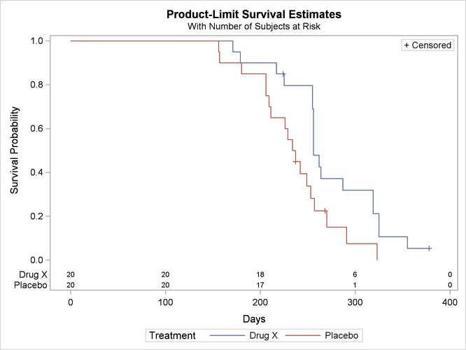
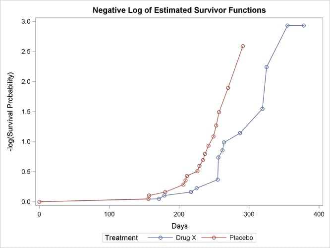
Figure 52.7 displays the graph of the log survivor function estimates versus survival time. Neither curve approximates a straight line through the origin—the exponential model is not appropriate for the survival data.
Note that these graphical displays are generated through ODS. For general information about ODS Graphics, see Chapter 21: Statistical Graphics Using ODS.
Figure 52.7: Plot of Estimated Negative Log Survivor Functions
Results of the comparison of survival curves between the two treatments are shown in Figure 52.8. The rank tests for homogeneity indicate a significant difference between the treatments (p = 0.0175 for the log-rank test and p = 0.0249 for the Wilcoxon test). Rats treated with Drug X live significantly longer than those treated with Placebo. Since the survival curves for the two treatments differ primarily at longer survival times, the Wilcoxon test, which places
more weight on shorter survival times, becomes less significant than the log-rank test. As noted earlier, the exponential
model is not appropriate for the given survival data; consequently, the result of the likelihood ratio test should be ignored.
Figure 52.8: Results of the Two-Sample Tests
| Test of Equality over Strata | |||
|---|---|---|---|
| Test | Chi-Square | DF | Pr > Chi-Square |
| Log-Rank | 5.6485 | 1 | 0.0175 |
| Wilcoxon | 5.0312 | 1 | 0.0249 |
| -2Log(LR) | 0.1983 | 1 | 0.6561 |
Next, suppose male rats and female rats are thought to have different survival rates, and you want to assess the treatment
effect while adjusting for the gender differences. By specifying the variable Sex in the STRATA statement as a stratifying variable and by specifying the variable Treatment in the GROUP= option, you can carry out a stratified test to test Treatment while adjusting for Sex. The test statistics are computed by pooling over the strata defined by the values of Sex, thus controlling for the effect of Sex. The NOTABLE option is added to the PROC LIFETEST statement as follows to avoid estimating a survival curve for each gender:
proc lifetest data=Exposed notable;
   time Days*Status(0);
   strata Sex / group=Treatment;
run;
Results of the stratified tests are shown in Figure 52.9. The treatment effect is statistically significant for both the log-rank test (p = 0.0071) and the Wilcoxon test (p = 0.0150). As compared to the results of the unstratified tests in Figure 52.8, the significance of the treatment effect has been sharpened by controlling for the effect of the gender of the subjects.
Figure 52.9: Results of the Stratified Two-Sample Tests
| Stratified Test of Equality over Group | |||
|---|---|---|---|
| Test | Chi-Square | DF | Pr > Chi-Square |
| Log-Rank | 7.2466 | 1 | 0.0071 |
| Wilcoxon | 5.9179 | 1 | 0.0150 |
Since Treatment is a binary variable, another way to study the effect of Treatment is to carry out a censored linear rank test with Treatment as an independent variable. This test is less popular than the two-sample test; nevertheless, in situations where the independent
variables are continuous and are difficult to discretize, it might be infeasible to perform a k-sample test. To compute the censored linear rank statistics to test the Treatment effect, Treatment is specified in the TEST statement as follows:
proc lifetest data=Exposed notable;
   time Days*Status(0);
   test Treatment;
run;
Results of the linear rank tests are shown Figure 52.10. The p-values are very similar to those of the two-sample tests in Figure 52.8.
Figure 52.10: Results of Linear Rank Tests of Treatment
| Univariate Chi-Squares for the Wilcoxon Test | ||||
|---|---|---|---|---|
| Variable | Test Statistic |
Standard Error |
Chi-Square | Pr > Chi-Square |
| Treatment | 3.9525 | 1.7524 | 5.0875 | 0.0241 |
| Univariate Chi-Squares for the Log-Rank Test | ||||
|---|---|---|---|---|
| Variable | Test Statistic |
Standard Error |
Chi-Square | Pr > Chi-Square |
| Treatment | 6.2708 | 2.6793 | 5.4779 | 0.0193 |
With Sex as a prognostic factor that you want to control, you can compute a stratified linear rank statistic to test the effect of
Treatment by specifying Sex in the STRATA statement and Treatment in the TEST statement as in the following program. The TEST=NONE option is specified in the STRATA statement to suppress
the two-sample tests for Sex.
proc lifetest data=Exposed notable;
   time Days*Status(0);
   strata Sex / test=none;
   test Treatment;
run;
Results of the stratified linear rank tests are shown in Figure 52.11. The p-values are very similar to those of the stratified tests in Figure 52.9.
Figure 52.11: Results of Stratified Linear Rank Tests of Treatment
| Univariate Chi-Squares for the Wilcoxon Test | ||||
|---|---|---|---|---|
| Variable | Test Statistic |
Standard Error |
Chi-Square | Pr > Chi-Square |
| Treatment | 4.2372 | 1.7371 | 5.9503 | 0.0147 |
| Univariate Chi-Squares for the Log-Rank Test | ||||
|---|---|---|---|---|
| Variable | Test Statistic |
Standard Error |
Chi-Square | Pr > Chi-Square |
| Treatment | 6.8021 | 2.5419 | 7.1609 | 0.0075 |