The KDE Procedure

Example 48.6 Bivariate KDE Graphics
This example illustrates the available bivariate graphics in PROC KDE. The octane data set comes from Rodriguez and Taniguchi (1980), where it is used for predicting customer octane satisfaction by using trained-rater observations. The variables in this
data set are Rater and Customer. Either variable might have missing values. See the file kdex3.sas in the SAS Sample Library. The following statements create the octane data set:
data octane;
   input Rater Customer;
   label Rater    = 'Rater'
         Customer = 'Customer';
   datalines;
94.5 92.0
94.0 88.0
94.0 90.0
93.0 93.0

   ... more lines ...

88.0 84.0
  .H 90.0
;
The following statements request all the available bivariate plots in PROC KDE:
ods graphics on;
proc kde data=octane;
   bivar Rater Customer / plots=all;
run;
ods graphics off;
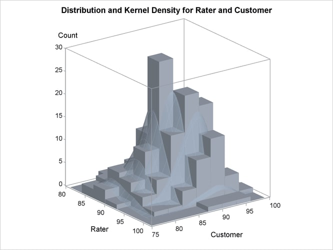
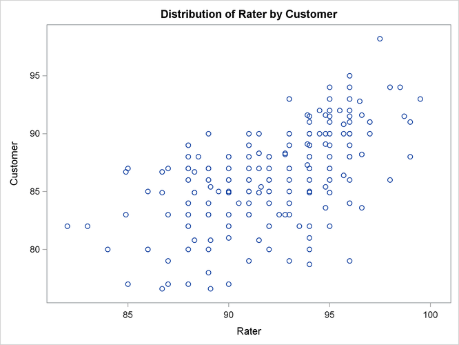
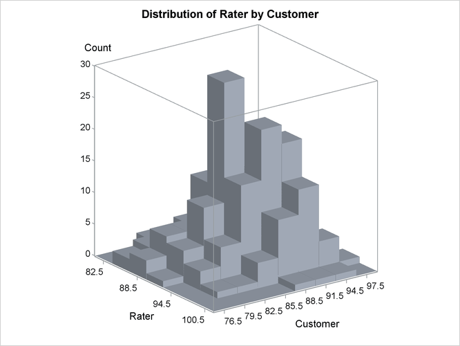
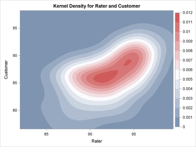
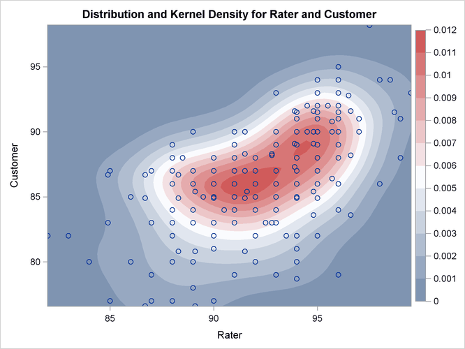
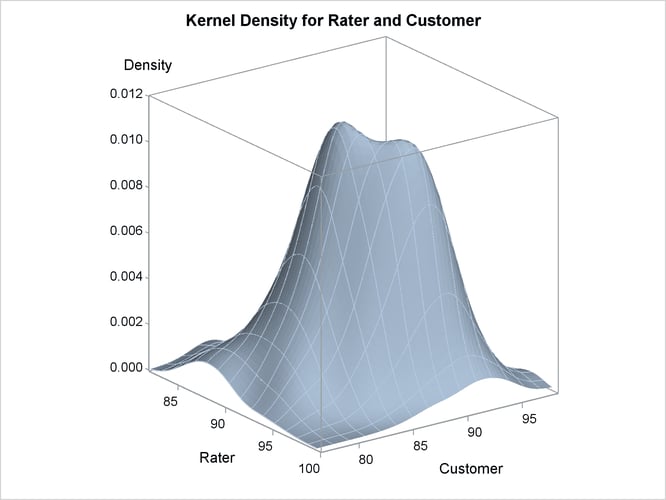
Output 48.6.1 shows a scatter plot of the data, Output 48.6.2 shows a bivariate histogram of the data, Output 48.6.3 shows a contour plot of bivariate density estimate, Output 48.6.4 shows a contour plot of bivariate density estimate overlaid with a scatter plot of data, Output 48.6.5 shows a surface plot of bivariate kernel density estimate, and Output 48.6.6 shows a bivariate histogram overlaid with a bivariate kernel density estimate. These graphical displays are requested by specifying the PLOTS= option in the BIVAR statement with ODS Graphics enabled. For general information about ODS Graphics, see Chapter 21: Statistical Graphics Using ODS. For specific information about the graphics available in the KDE procedure, see the section ODS Graphics.
Output 48.6.1: Scatter Plot
Output 48.6.2: Bivariate Histogram
Output 48.6.3: Contour Plot
Output 48.6.4: Contour Plot with Overlaid Scatter Plot
Output 48.6.5: Surface Plot
Output 48.6.6: Bivariate Histogram with Overlaid Surface Plot