The GLM Procedure
-
Overview

-
Getting Started
-
Syntax
-
DetailsStatistical Assumptions for Using PROC GLMSpecification of EffectsUsing PROC GLM InteractivelyParameterization of PROC GLM ModelsHypothesis Testing in PROC GLMEffect Size Measures for F Tests in GLMAbsorptionSpecification of ESTIMATE ExpressionsComparing GroupsMultivariate Analysis of VarianceRepeated Measures Analysis of VarianceRandom-Effects AnalysisMissing ValuesComputational ResourcesComputational MethodOutput Data SetsDisplayed OutputODS Table NamesODS Graphics
-
ExamplesRandomized Complete Blocks with Means Comparisons and ContrastsRegression with Mileage DataUnbalanced ANOVA for Two-Way Design with InteractionAnalysis of CovarianceThree-Way Analysis of Variance with ContrastsMultivariate Analysis of VarianceRepeated Measures Analysis of VarianceMixed Model Analysis of Variance with the RANDOM StatementAnalyzing a Doubly Multivariate Repeated Measures DesignTesting for Equal Group VariancesAnalysis of a Screening Design
- References
Example 42.2 Regression with Mileage Data
A car is tested for gas mileage at various speeds to determine at what speed the car achieves the highest gas mileage. A quadratic model is fit to the experimental data. The following statements produce Output 42.2.1 through Output 42.2.4.
title 'Gasoline Mileage Experiment';
data mileage;
   input mph mpg @@;
   datalines;
20 15.4
30 20.2
40 25.7
50 26.2  50 26.6  50 27.4
55   .
60 24.8
;
ods graphics on;
proc glm;
   model mpg=mph mph*mph / p clm;
run;
ods graphics off;
Output 42.2.1: Standard Regression Analysis
| Gasoline Mileage Experiment |
| Number of Observations Read | 8 |
|---|---|
| Number of Observations Used | 7 |
| Gasoline Mileage Experiment |
| Source | DF | Sum of Squares | Mean Square | F Value | Pr > F |
|---|---|---|---|---|---|
| Model | 2 | 111.8086183 | 55.9043091 | 77.96 | 0.0006 |
| Error | 4 | 2.8685246 | 0.7171311 | ||
| Corrected Total | 6 | 114.6771429 |
| R-Square | Coeff Var | Root MSE | mpg Mean |
|---|---|---|---|
| 0.974986 | 3.564553 | 0.846836 | 23.75714 |
| Source | DF | Type I SS | Mean Square | F Value | Pr > F |
|---|---|---|---|---|---|
| mph | 1 | 85.64464286 | 85.64464286 | 119.43 | 0.0004 |
| mph*mph | 1 | 26.16397541 | 26.16397541 | 36.48 | 0.0038 |
| Source | DF | Type III SS | Mean Square | F Value | Pr > F |
|---|---|---|---|---|---|
| mph | 1 | 41.01171219 | 41.01171219 | 57.19 | 0.0016 |
| mph*mph | 1 | 26.16397541 | 26.16397541 | 36.48 | 0.0038 |
| Parameter | Estimate | Standard Error | t Value | Pr > |t| |
|---|---|---|---|---|
| Intercept | -5.985245902 | 3.18522249 | -1.88 | 0.1334 |
| mph | 1.305245902 | 0.17259876 | 7.56 | 0.0016 |
| mph*mph | -0.013098361 | 0.00216852 | -6.04 | 0.0038 |
The overall F statistic is significant. The tests of mph and mph*mph in the Type I sums of squares show that both the linear and quadratic terms in the regression model are significant. The
model fits well, with an R square of 0.97. The table of parameter estimates indicates that the estimated regression equation
is
|
|
|
|
Output 42.2.2: Results of Requesting the P and CLM Options
| Observation | Observed | Predicted | Residual | 95% Confidence Limits for Mean Predicted Value |
||
|---|---|---|---|---|---|---|
| 1 | 15.40000000 | 14.88032787 | 0.51967213 | 12.69701317 | 17.06364257 | |
| 2 | 20.20000000 | 21.38360656 | -1.18360656 | 20.01727192 | 22.74994119 | |
| 3 | 25.70000000 | 25.26721311 | 0.43278689 | 23.87460041 | 26.65982582 | |
| 4 | 26.20000000 | 26.53114754 | -0.33114754 | 25.44573423 | 27.61656085 | |
| 5 | 26.60000000 | 26.53114754 | 0.06885246 | 25.44573423 | 27.61656085 | |
| 6 | 27.40000000 | 26.53114754 | 0.86885246 | 25.44573423 | 27.61656085 | |
| 7 | * | . | 26.18073770 | . | 24.88679308 | 27.47468233 |
| 8 | 24.80000000 | 25.17540984 | -0.37540984 | 23.05954977 | 27.29126990 | |
The P and CLM options in the MODEL statement produce the table shown in Output 42.2.2. For each observation, the observed, predicted, and residual values are shown. In addition, the 95% confidence limits for
a mean predicted value are shown for each observation. Note that the observation with a missing value for mph is not used in the analysis, but predicted and confidence limit values are shown.
Output 42.2.3: Additional Results of Requesting the P and CLM Options
| Sum of Residuals | -0.00000000 |
|---|---|
| Sum of Squared Residuals | 2.86852459 |
| Sum of Squared Residuals - Error SS | -0.00000000 |
| PRESS Statistic | 23.18107335 |
| First Order Autocorrelation | -0.54376613 |
| Durbin-Watson D | 2.94425592 |
The last portion of the output listing, shown in Output 42.2.3, gives some additional information about the residuals. The Press statistic gives the sum of squares of predicted residual errors, as described in Chapter 4: Introduction to Regression Procedures. The First Order Autocorrelation and the Durbin-Watson D statistic, which measures first-order autocorrelation, are also given.
Output 42.2.4: Plot of Mileage Data
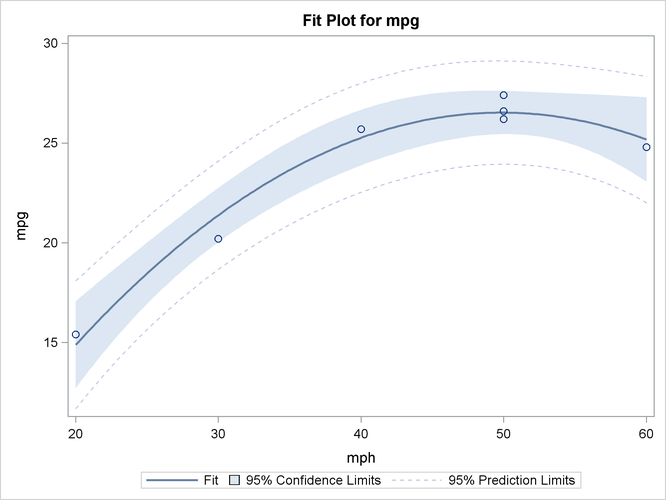
Finally, the ODS GRAPHICS ON command in the previous statements enables ODS Graphics, which in this case produces the plot
shown in Output 42.2.4 of the actual and predicted values for the data, as well as a band representing the confidence limits for individual predictions.
The quadratic relationship between mpg and mph is evident.