The SURVEYFREQ Procedure

Rao-Scott Chi-Square Test
The Rao-Scott chi-square test is a design-adjusted version of the Pearson chi-square test, which involves differences between observed and expected frequencies. See Lohr (2009, Section 10.3.2), Rao and Scott (1981, 1984, 1987), and Thomas, Singh, and Roberts (1996) for information about design-adjusted chi-square tests.
PROC SURVEYFREQ provides a first-order Rao-Scott chi-square test by default. If you specify the CHISQ(SECONDORDER) option, PROC SURVEYFREQ provides a second-order (Satterthwaite) Rao-Scott chi-square test. The first-order design correction depends only on the design effects of the table cell proportion estimates and, for two-way tables, the design effects of the marginal proportion estimates. The second-order design correction requires computation of the full covariance matrix of the proportion estimates. The second-order test requires more computational resources than the first-order test, but it can provide some performance advantages (for Type I error and power), particularly when the design effects are variable (Thomas and Rao 1987; Rao and Thomas 1989).
One-Way Tables
For one-way tables, the CHISQ option provides a Rao-Scott (design-based) goodness-of-fit test for one-way tables. By default, this is a test for the null hypothesis of equal proportions. If you specify null hypothesis proportions in the TESTP= option, the goodness-of-fit test uses the specified proportions.
First-Order Test
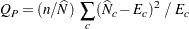
The first-order Rao-Scott chi-square statistic for the goodness-of-fit test is computed as
 |
where  is the Pearson chi-square based on the estimated totals and
  is the first-order design correction described in the section First-Order Design Correction. See Rao and Scott (1979, 1981, and 1984) for details.
For a one-way table with  levels, the Pearson chi-square is computed as
 |
where  is the sample size,
  is the estimated overall total,
  is the estimated total for level
  , and
, and  is the expected total for level under the null hypothesis. For the null hypothesis of equal proportions, the expected total for each level is
 |
For specified null proportions, the expected total for level equals
 |
where  is the null proportion that you specify for level .
Under the null hypothesis, the first-order Rao-Scott chi-square  approximately follows a chi-square distribution with
  degrees of freedom. A better approximation can be obtained by the
  statistic,
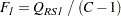 |
which has an distribution with and  degrees of freedom under the null hypothesis (Thomas and Rao 1984, 1987). The value of
  is the degrees of freedom for the variance estimator, which depends on the sample design and the variance estimation method. The section Degrees of Freedom describes the computation of .
First-Order Design Correction
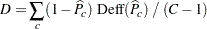
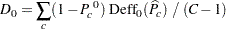
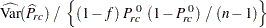
By default for one-way tables, the first-order design correction is computed from the proportion estimates as
 |
where
 |
 |
 |
|||
 |
|
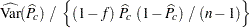 |
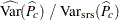
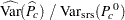
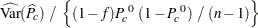
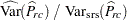
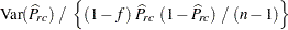
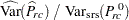
as described in the section Design Effect.  is the proportion estimate for level ,
  is the variance of the estimate,
  is the overall sampling fraction, and is the number of observations in the sample. The factor
  is included only for Taylor series variance estimation (VARMETHOD=TAYLOR) when you specify the RATE= or TOTAL= option. See the section Design Effect for details.
If you specify the CHISQ(MODIFIED) or LRCHISQ(MODIFIED) option, the design correction is computed by using null hypothesis proportions instead of proportion estimates. By default, null hypothesis proportions are equal proportions for all levels of the one-way table. Alternatively, you can specify null proportion values in the TESTP= option. The modified design correction  is computed from null hypothesis proportions as
 |
where
 |
|
 |
|||
|
|
 |
The null hypothesis proportion equals  for equal proportions (the default), or equals the null proportion that you specify for level if you use the TESTP= option.
Second-Order Test
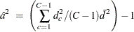
The second-order (Satterthwaite) Rao-Scott chi-square statistic for the goodness-of-fit test is computed as
 |
where is the first-order Rao-Scott chi-square statistic described in the section First-Order Test and  is the second-order design correction described in the section Second-Order Design Correction. See Rao and Scott (1979, 1981) and Rao and Thomas (1989) for details.
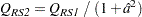
Under the null hypothesis, the second-order Rao-Scott chi-square  approximately follows a chi-square distribution with
  degrees of freedom. The corresponding statistic is
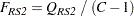 |
which has an distribution with and 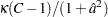 degrees of freedom under the null hypothesis (Thomas and Rao 1984, 1987). The value of is the degrees of freedom for the variance estimator, which depends on the sample design and the variance estimation method. The section Degrees of Freedom describes the computation of .
Second-Order Design Correction
The second-order (Satterthwaite) design correction for one-way tables is computed from the eigenvalues of the estimated design effects matrix  , which are known as generalized design effects. The design effects matrix is computed as
 |
where  is the covariance under multinomial sampling (srs with replacement) and
  is the covariance matrix of the first proportion estimates. See Rao and Scott (1979, 1981) and Rao and Thomas (1989) for details.
By default, the srs covariance matrix is computed from the proportion estimates as
 |
where  is the array of the first proportion estimates. If you specify the CHISQ(MODIFIED) or LRCHISQ(MODIFIED) option, the srs covariance matrix is computed from the null hypothesis proportions
  as
as
 |
where is the array of the first null hypothesis proportions. The null hypothesis proportions equal by default. If you use the TESTP= option to specify null hypothesis proportions, is the array of the first proportions that you specify.
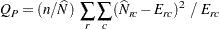
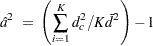
The second-order design correction is computed as
 |
where  are the eigenvalues of the design effects matrix and
  is the average of the eigenvalues.
Two-Way Tables
For two-way tables, the CHISQ option provides a Rao-Scott (design-based) test of association between the row and column variables. PROC SURVEYFREQ provides a first-order Rao-Scott chi-square test by default. If you specify the CHISQ(SECONDORDER) option, PROC SURVEYFREQ provides a second-order (Satterthwaite) Rao-Scott chi-square test.
First-Order Test
The first-order Rao-Scott chi-square statistic is computed as
|
where is the Pearson chi-square based on the estimated totals and is the design correction described in the section First-Order Design Correction. See Rao and Scott (1979, 1984, and 1987) for details.
For a two-way tables with  rows and columns, the Pearson chi-square is computed as
 |
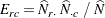
where is the sample size, is the estimated overall total,  is the estimated total for table cell
  , and
, and  is the expected total for table cell under the null hypothesis of no association,
 |
Under the null hypothesis of no association, the first-order Rao-Scott chi-square approximately follows a chi-square distribution with  degrees of freedom. A better approximation can be obtained by the statistic,
 |
which has an distribution with and  degrees of freedom under the null hypothesis (Thomas and Rao 1984, 1987). The value of is the degrees of freedom for the variance estimator, which depends on the sample design and the variance estimation method. The section Degrees of Freedom describes the computation of .
First-Order Design Correction
By default for a first-order test, PROC SURVEYFREQ computes the design correction from proportion estimates. If you specify the CHISQ(MODIFIED) or LRCHISQ(MODIFIED) option for a first-order test, the procedure computes the design correction from null hypothesis proportions.
Second-order tests, which you request by specifying the CHISQ(SECONDORDER) or LRCHISQ(SECONDORDER) option, are computed by applying both first-order and second-order design corrections to the weighted chi-square statistic. For second-order tests for two-way tables, PROC SURVEYFREQ always uses null hypothesis proportions to compute both the first-order and second-order design corrections.
The first-order design correction that is based on proportion estimates is computed as
 |
 |
|||
|
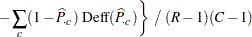 |
where
 |
|
 |
|||
|
|
 |
as described in the section Design Effect.  is the estimate of the proportion in table cell
  ,
,  is the variance of the estimate, is the overall sampling fraction, and is the number of observations in the sample. The factor is included only for Taylor series variance estimation (VARMETHOD=TAYLOR) when you specify the RATE= or TOTAL= option. See the section Design Effect for details.
The design effects for the estimate of the proportion in row  and the estimate of the proportion in column (
 and
and  , respectively) are computed in the same way.
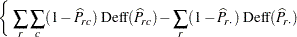
If you specify the CHISQ(MODIFIED) or LRCHISQ(MODIFIED) option for a first-order Rao-Scott test, or if you request a second-order test for a two-way table (CHISQ(SECONDORDER) or LRCHISQ(MODIFIED)), the procedure computes the design correction from the null hypothesis cell proportions instead of the estimated cell proportions. For two-way tables, the null hypothesis cell proportions are computed as the products of the corresponding row and column proportion estimates. The modified design correction (based on null hypothesis proportions) is computed as
 |
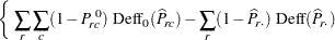 |
|||
|
|
where
 |
and
 |
|
 |
|||
|
|
 |
Second-Order Test
The second-order (Satterthwaite) Rao-Scott chi-square statistic for two-way tables is computed as
|
where is the first-order Rao-Scott chi-square statistic described in the section First-Order Test and is the second-order design correction described in the section Second-Order Design Correction. See Rao and Scott (1979, 1981) and Rao and Thomas (1989) for details.
Under the null hypothesis, the second-order Rao-Scott chi-square approximately follows a chi-square distribution with 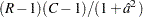 degrees of freedom. The corresponding statistic is
 |
which has an distribution with and 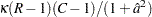 degrees of freedom under the null hypothesis (Thomas and Rao 1984, 1987). The value of is the degrees of freedom for the variance estimator, which depends on the sample design and the variance estimation method. The section Degrees of Freedom describes the computation of .
Second-Order Design Correction
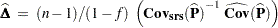
The second-order (Satterthwaite) design correction for two-way tables is computed from the eigenvalues of the estimated design effects matrix , which are known as generalized design effects. The design effects matrix is defined as
 |
where is the covariance matrix of the  proportion estimates and is the covariance under multinomial sampling (srs with replacement). See Rao and Scott (1979, 1981) and Rao and Thomas (1989) for details.
The second-order design correction is computed from the design effects matrix as
 |
where 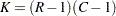 , are the eigenvalues of , and is the average eigenvalue.
The srs covariance matrix is computed as
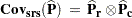 |
where  is an
is an 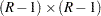 matrix that is constructed from the
  array of row proportion estimates
  as
as
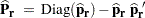 |
Similarly,  is an
is an 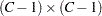 matrix that is constructed from the array of column proportion estimates
  as
as
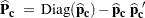 |
The  matrix
  is computed as
 |
where  ,
,  ,
,  is an
is an  array of ones, and
  is an
is an  array of ones. See Rao and Scott (1979, page 61) for details.