The STDIZE Procedure

Getting Started: STDIZE Procedure
The following example demonstrates how you can use the STDIZE procedure to obtain location and scale measures of your data.
In the following hypothetical data set, a random sample of grade twelve students is selected from a number of coeducational schools. Each school is classified as one of two types: Urban or Rural. There are 40 observations.
The variables are id (student identification), Type (type of school attended: ‘urban’=urban area and ‘rural’=rural area), and total (total assessment scores in History, Geometry, and Chemistry).
The following DATA step creates the SAS data set TotalScores.
data TotalScores;
   title 'High School Scores Data';
   input id Type $ total @@;
   datalines;
 1 rural 135   2 rural 125   3 rural 223   4 rural 224   5 rural 133
 6 rural 253   7 rural 144   8 rural 193   9 rural 152  10 rural 178
11 rural 120  12 rural 180  13 rural 154  14 rural 184  15 rural 187
16 rural 111  17 rural 190  18 rural 128  19 rural 110  20 rural 217
21 urban 192  22 urban 186  23 urban  64  24 urban 159  25 urban 133
26 urban 163  27 urban 130  28 urban 163  29 urban 189  30 urban 144
31 urban 154  32 urban 198  33 urban 150  34 urban 151  35 urban 152
36 urban 151  37 urban 127  38 urban 167  39 urban 170  40 urban 123
;
Suppose you now want to standardize the total scores in different types of schools prior to any further analysis. Before standardizing the total scores, you can use the box plot from PROC BOXPLOT to summarize the total scores for both types of schools.
ods graphics on;
proc boxplot data=TotalScores;
   plot total*Type / boxstyle=schematic noserifs;
run;
The PLOT statement in the PROC BOXPLOT statement creates the schematic plots (without the serifs) when you specify boxstyle=schematic noserifs. Figure 84.1 displays a box plot for each type of school.
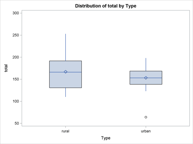
Inspection reveals that one urban score is a low outlier. Also, if you compare the lengths of two box plots, there seems to be twice as much dispersion for the rural scores as for the urban scores.
The following PROC UNIVARIATE statement reports the information about the extreme values of the Score variable for each type of school:
proc univariate data=TotalScores;
   var total;
   by Type;
run;
Figure 84.2 displays the table from PROC UNIVARIATE for the lowest and highest five total scores for urban schools. The outlier (Obs = 23), marked in Figure 84.2 by the symbol '0', has a score of 64.
| High School Scores Data |
| Extreme Observations | |||
|---|---|---|---|
| Lowest | Highest | ||
| Value | Obs | Value | Obs |
| 64 | 23 | 170 | 39 |
| 123 | 40 | 186 | 22 |
| 127 | 37 | 189 | 29 |
| 130 | 27 | 192 | 21 |
| 133 | 25 | 198 | 32 |
The following PROC STDIZE procedure requests the METHOD=STD option for computing the location and scale measures:
proc stdize data=totalscores method=std pstat;
   title2 'METHOD=STD';
   var total;
   by Type;
run;
Figure 84.3 displays the table of location and scale measures from the PROC STDIZE statement. PROC STDIZE uses the sample mean as the location measure and the sample standard deviation as the scale measure for standardizing. The PSTAT option displays a table containing these two measures.
| High School Scores Data |
| METHOD=STD |
| Location and Scale Measures | |||
|---|---|---|---|
| Location = mean Scale = standard deviation | |||
| Name | Location | Scale | N |
| total | 167.050000 | 41.956713 | 20 |
| High School Scores Data |
| METHOD=STD |
| Location and Scale Measures | |||
|---|---|---|---|
| Location = mean Scale = standard deviation | |||
| Name | Location | Scale | N |
| total | 153.300000 | 30.066768 | 20 |
The ratio of the scale of rural scores to the scale of urban scores is approximately 1.4 (41.96/30.07). This ratio is smaller than the dispersion ratio observed in the previous schematic plots.
The STDIZE procedure provides several location and scale measures that are resistant to outliers. The following statements invoke three different standardization methods and display the tables for the location and scale measures:
proc stdize data=totalscores method=mad pstat;
   title2 'METHOD=MAD';
   var total;
   by Type;
run;
proc stdize data=totalscores method=iqr pstat;
   title2 'METHOD=IQR';
   var total;
   by Type;
run;
proc stdize data=totalscores method=abw(4) pstat;
   title2 'METHOD=ABW(4)';
   var total;
   by Type;
run;
Figure 84.4 displays the table of location and scale measures when the standardization method is median absolute deviation (MAD). The location measure is the median, and the scale measure is the median absolute deviation from the median. The ratio of the scale of rural scores to the scale of urban scores is approximately 2.06 (32.0/15.5) and is close to the dispersion ratio observed in the previous schematic plots.
| High School Scores Data |
| METHOD=MAD |
| Location and Scale Measures | |||
|---|---|---|---|
| Location = median Scale = median abs dev from median |
|||
| Name | Location | Scale | N |
| total | 166.000000 | 32.000000 | 20 |
| High School Scores Data |
| METHOD=MAD |
| Location and Scale Measures | |||
|---|---|---|---|
| Location = median Scale = median abs dev from median |
|||
| Name | Location | Scale | N |
| total | 153.000000 | 15.500000 | 20 |
Figure 84.5 displays the table of location and scale measures when the standardization method is IQR. The location measure is the median, and the scale measure is the interquartile range. The ratio of the scale of rural scores to the scale of urban scores is approximately 2.03 (61/30) and is, in fact, the dispersion ratio observed in the previous schematic plots.
| High School Scores Data |
| METHOD=IQR |
| Location and Scale Measures | |||
|---|---|---|---|
| Location = median Scale = interquartile range |
|||
| Name | Location | Scale | N |
| total | 166.000000 | 61.000000 | 20 |
| High School Scores Data |
| METHOD=IQR |
| Location and Scale Measures | |||
|---|---|---|---|
| Location = median Scale = interquartile range |
|||
| Name | Location | Scale | N |
| total | 153.000000 | 30.000000 | 20 |
Figure 84.6 displays the table of location and scale measures when the standardization method is ABW, for which the location measure is the biweight one-step M-estimate, and the scale measure is the biweight A-estimate. Note that the initial estimate for ABW is MAD. The following steps help to decide the value of the tuning constant:
For rural scores, the location estimate for MAD is 166.0, and the scale estimate for MAD is 32.0. The maximum of the rural scores is 253 (not shown), and the minimum is 110 (not shown). Thus, the tuning constant needs to be 3 so that it does not reject any observation that has a score between 110 to 253.
For urban scores, the location estimate for MAD is 153.0, and the scale estimate for MAD is 15.5. The maximum of the rural scores is 198, and the minimum (also an outlier) is 64. Thus, the tuning constant needs to be 4 so that it rejects the outlier (64) but includes the maximum (198) as an normal observation.
The maximum of the tuning constants, obtained in steps 1 and 2, is 4.
See Goodall (1983, Chapter 11) for details about the tuning constant. The ratio of the scale of rural scores to the scale of urban scores is approximately 2.06 (32.0/15.5). It is also close to the dispersion ratio observed in the previous schematic plots.
| High School Scores Data |
| METHOD=ABW(4) |
| Location and Scale Measures | |||
|---|---|---|---|
| Location = biweight 1-step M-estimate Scale = biweight A-estimate |
|||
| Name | Location | Scale | N |
| total | 162.889603 | 56.662855 | 20 |
| High School Scores Data |
| METHOD=ABW(4) |
| Location and Scale Measures | |||
|---|---|---|---|
| Location = biweight 1-step M-estimate Scale = biweight A-estimate |
|||
| Name | Location | Scale | N |
| total | 156.014608 | 28.615980 | 20 |
The preceding analysis shows that METHOD=MAD, METHOD=IQR, and METHOD=ABW all provide better dispersion ratios than METHOD=STD does.
You can recompute the standard deviation after deleting the outlier from the original data set for comparison. The following statements create a data set NoOutlier that excludes the outlier from the TotalScores data set and invoke PROC STDIZE with METHOD=STD.
data NoOutlier;
   set totalscores;
   if (total = 64) then delete;
run;
proc stdize data=NoOutlier method=std pstat;
   title2 'After Removing Outlier, METHOD=STD';
   var total;
   by Type;
run;
Figure 84.7 displays the location and scale measures after deleting the outlier. The lack of resistance of the standard deviation to outliers is clearly illustrated: if you delete the outlier, the sample standard deviation of urban scores changes from 30.07 to 22.09. The new ratio of the scale of rural scores to the scale of urban scores is approximately 1.90 (41.96/22.09).
| High School Scores Data |
| After Removing Outlier, METHOD=STD |
| Location and Scale Measures | |||
|---|---|---|---|
| Location = mean Scale = standard deviation | |||
| Name | Location | Scale | N |
| total | 167.050000 | 41.956713 | 20 |
| High School Scores Data |
| After Removing Outlier, METHOD=STD |
| Location and Scale Measures | |||
|---|---|---|---|
| Location = mean Scale = standard deviation | |||
| Name | Location | Scale | N |
| total | 158.000000 | 22.088207 | 19 |