The RSREG Procedure

| Searching for Multiple Response Conditions |
Suppose you have the following data with two factors and three responses, and you want to find the factor setting that produces responses in a certain region:
data a;
   input x1 x2 y1 y2 y3;
   datalines;
-1      -1         1.8 1.940  3.6398
-1       1         2.6 1.843  4.9123
 1      -1         5.4 1.063  6.0128
 1       1         0.7 1.639  2.3629
 0       0         8.5 0.134  9.0910
 0       0         3.0 0.545  3.7349
 0       0         9.8 0.453 10.4412
 0       0         4.1 1.117  5.0042
 0       0         4.8 1.690  6.6245
 0       0         5.9 1.165  6.9420
 0       0         7.3 1.013  8.7442
 0       0         9.3 1.179 10.2762
 1.4142  0         3.9 0.945  5.0245
-1.4142  0         1.7 0.333  2.4041
 0       1.4142    3.0 1.869  5.2695
 0      -1.4142    5.7 0.099  5.4346
;
You want to find the values of x1 and x2 that maximize y1 subject to y2<2 and y3<y2+y1. The exact answer is not easy to obtain analytically, but you can obtain a practically feasible solution by checking conditions across a grid of values in the range of interest. First, append a grid of factor values to the observed data, with missing values for the responses:
data b;
   set a end=eof;
   output;
   if eof then do;
      y1=.;
      y2=.;
      y3=.;
      do x1=-2 to 2 by .1;
         do x2=-2 to 2 by .1;
            output;
         end;
      end;
   end;
run;
Next, use PROC RSREG to fit a response surface model to the data and to compute predicted values for both the observed data and the grid, putting the predicted values in a data set c:
proc rsreg data=b out=c;
   model y1 y2 y3=x1 x2 / predict;
run;
Finally, find the subset of predicted values that satisfy the constraints, sort by the unconstrained variable, and display the top five predictions:
data d;
   set c;
   if y2<2;
   if y3<y2+y1;

proc sort data=d;
   by descending y1;
run;

data d; set d;
   if (_n_ <= 5);
proc print;
run;
The results are displayed in Figure 78.5. They indicate that optimal values of the factors are around 0.3 for x1 and around –0.5 for x2.
| Obs | x1 | x2 | _TYPE_ | y1 | y2 | y3 |
|---|---|---|---|---|---|---|
| 1 | 0.3 | -0.5 | PREDICT | 6.92570 | 0.75784 | 7.60471 |
| 2 | 0.3 | -0.6 | PREDICT | 6.91424 | 0.74174 | 7.54194 |
| 3 | 0.3 | -0.4 | PREDICT | 6.91003 | 0.77870 | 7.64341 |
| 4 | 0.4 | -0.6 | PREDICT | 6.90769 | 0.73357 | 7.51836 |
| 5 | 0.4 | -0.5 | PREDICT | 6.90540 | 0.75135 | 7.56883 |
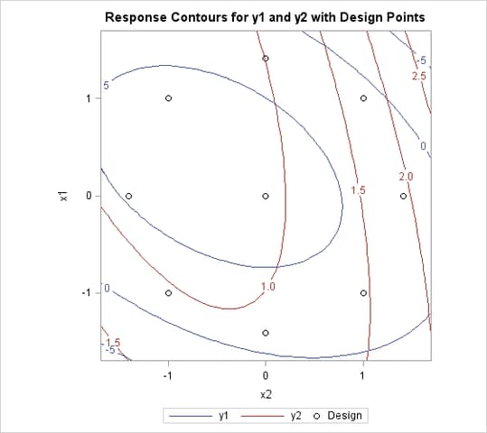
If you are also interested in simultaneously optimizing y1 and y2, you can specify the following statements to make a visual comparison of the two response surfaces by overlaying their contour plots:
ods graphics on;
proc rsreg data=a plots=surface(overlaypairs);
   model y1 y2=x1 x2;
run;
ods graphics off;
Figure 78.6 shows that you have to make some compromises in any attempt to maximize both y1 and y2; however, you might be able to maximize y1 while minimizing y2.