The ROBUSTREG Procedure

| ODS Graphics |
Statistical procedures use ODS Graphics to create graphs as part of their output. ODS Graphics is described in detail in Chapter 21, Statistical Graphics Using ODS.
Before you create graphs, ODS Graphics must be enabled (for example, with the ODS GRAPHICS ON statement). For more information about enabling and disabling ODS Graphics, see the section Enabling and Disabling ODS Graphics in Chapter 21, Statistical Graphics Using ODS.
The overall appearance of graphs is controlled by ODS styles. Styles and other aspects of using ODS Graphics are discussed in the section A Primer on ODS Statistical Graphics in Chapter 21, Statistical Graphics Using ODS.
If the model includes a single continuous independent variable, a plot of robust fit against this variable (FITPLOT) is provided by default. Two plots are particularly useful in revealing outliers and leverage points. The first is a scatter plot of the standardized robust residuals against the robust distances (RDPLOT). The second is a scatter plot of the robust distances against the classical Mahalanobis distances (DDPLOT). In addition to these two plots, a histogram and a quantile-quantile plot of the standardized robust residuals are also helpful.
PROC ROBUSTREG assigns a name to each graph it creates using ODS. You can use these names to refer to the graphs when using ODS. The names and PLOTS= options are listed in Table 77.10.
ODS Graph Name |
Plot Description |
Statement |
PLOTS= Option |
|---|---|---|---|
DDPlot |
Robust distance versus Mahalanobis distance (or projected robust distance versus Projected Mahalanobis distance) |
PROC |
DDPLOT |
FitPlot |
Robust fit versus independent variable |
PROC |
FITPLOT |
Histogram |
Histogram of standardized robust residuals |
PROC |
HISTOGRAM |
QQPlot |
Q-Q plot of standardized robust residuals |
PROC |
QQPLOT |
RDPlot |
Standardized robust residual versus robust distance (or projected robust distance) |
PROC |
RDPLOT |
Fit Plot
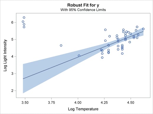
When the model has a single independent continuous variable (with or without the intercept), the ROBUSTREG procedure automatically creates a plot of robust fit against this independent variable.
The following simple example shows the fit plot. The data, from Rousseeuw and Leroy (1987, Table 3), include the logarithm of surface temperature and the logarithm of light intensity for 47 stars in the direction of the constellation Cygnus.
data star;
   input index x y @@;
   label x = 'Log Temperature'
         y = 'Log Light Intensity';
   datalines;
1   4.37  5.23     25  4.38  5.02
2   4.56  5.74     26  4.42  4.66
3   4.26  4.93     27  4.29  4.66
4   4.56  5.74     28  4.38  4.90
5   4.30  5.19     29  4.22  4.39
6   4.46  5.46     30  3.48  6.05
7   3.84  4.65     31  4.38  4.42
8   4.57  5.27     32  4.56  5.10
9   4.26  5.57     33  4.45  5.22
10  4.37  5.12     34  3.49  6.29
11  3.49  5.73     35  4.23  4.34
12  4.43  5.45     36  4.62  5.62
13  4.48  5.42     37  4.53  5.10
14  4.01  4.05     38  4.45  5.22
15  4.29  4.26     39  4.53  5.18
16  4.42  4.58     40  4.43  5.57
17  4.23  3.94     41  4.38  4.62
18  4.42  4.18     42  4.45  5.06
19  4.23  4.18     43  4.50  5.34
20  3.49  5.89     44  4.45  5.34
21  4.29  4.38     45  4.55  5.54
22  4.29  4.22     46  4.45  4.98
23  4.42  4.42     47  4.42  4.50
24  4.49  4.85
;
The following statements plot the robust fit of the logarithm of light intensity with the MM method against the logarithm of the surface temperature.
ods graphics on;

proc robustreg data=star method=mm ;
    model y = x;
run;
Figure 77.22 shows the fit plot. Confidence limits are added on the plot by default.
You can suppress the confidence limits with the NOLIMITS option, as shown in the following statements:
proc robustreg data=star method=mm plot=fitplot(nolimits);
    model y = x;
run;
Distance-Distance Plot
The distance-distance plot (DDPLOT) is mainly used for leverage-point diagnostics. It is a scatter plot of the robust distances (or projected robust distances) against the classical Mahalanobis distances (or projected classical Mahalanobis distances) for the independent variables. See the section Leverage Point and Outlier Detection for details about the robust distance.
You can use the PLOT=DDPLOT option to request this plot. The following statements use the stack data set in the section M Estimation to create the single plot shown in Figure 77.5.
proc robustreg data=stack plot=ddplot;
   model y = x1 x2 x3;
run;
The reference lines represent the cutoff values. The diagonal line is also drawn to show the distribution of the distances. By default, all outliers and leverage points are labeled with observation numbers. To change the default, you can use the LABEL= option as described in Table 77.1.
If you specify ID variables in the ID statement, the values of the first ID variable instead of observation numbers are used as labels.
Residual-Distance Plot
The residual-distance plot (RDPLOT) is used for both outlier and leverage-point diagnostics. It is a scatter plot of the standardized robust residuals against the robust distances. See the section Leverage Point and Outlier Detection for details about the robust distance.
You can use the PLOT=RDPLOT option to request this plot. The following statements use the stack data set in the section M Estimation to create the plot shown in Figure 77.4.
proc robustreg data=stack plot=rdplot;
   model y = x1 x2 x3;
run;
The reference lines represent the cutoff values. By default, all outliers and leverage points are labeled with observation numbers. To change the default, you can use the LABEL= option as described in Table 77.1.
If you specify ID variables in the ID statement, the values of the first ID variable instead of observation numbers are used as labels.
Histogram and Q-Q Plot
PROC ROBUSTREG produces a histogram and a Q-Q plot for the standardized robust residuals. The histogram is superimposed with a normal density curve and a kernel density curve. Using the stack data set in the section M Estimation, the following statements create the plots in Figure 77.6 and Figure 77.7.
proc robustreg data=stack plots=(histogram qqplot);
   model y = x1 x2 x3;
run;