The POWER Procedure
- Overview
-
Getting Started

-
Syntax
PROC POWER Statement LOGISTIC Statement MULTREG Statement ONECORR Statement ONESAMPLEFREQ Statement ONESAMPLEMEANS Statement ONEWAYANOVA Statement PAIREDFREQ Statement PAIREDMEANS Statement PLOT Statement TWOSAMPLEFREQ Statement TWOSAMPLEMEANS Statement TWOSAMPLESURVIVAL Statement TWOSAMPLEWILCOXON Statement
-
Details
Overview of Power Concepts Summary of Analyses Specifying Value Lists in Analysis Statements Sample Size Adjustment Options Error and Information Output Displayed Output ODS Table Names Computational Resources Computational Methods and Formulas ODS Graphics ODS Styles Suitable for Use with PROC POWER
-
Examples
One-Way ANOVA The Sawtooth Power Function in Proportion Analyses Simple AB/BA Crossover Designs Noninferiority Test with Lognormal Data Multiple Regression and Correlation Comparing Two Survival Curves Confidence Interval Precision Customizing Plots Binary Logistic Regression with Independent Predictors Wilcoxon-Mann-Whitney Test
- References
Example 70.2 The Sawtooth Power Function in Proportion Analyses
For many common statistical analyses, the power curve is monotonically increasing: the more samples you take, the more power you achieve. However, in statistical analyses of discrete data, such as tests of proportions, the power curve is often nonmonotonic. A small increase in sample size can result in a decrease in power, a decrease that is sometimes substantial. The explanation is that the actual significance level (in other words, the achieved Type I error rate) for discrete tests strays below the target level and varies with sample size. The power loss from a decrease in the Type I error rate can outweigh the power gain from an increase in sample size. The example discussed here demonstrates this "sawtooth" phenomenon. For additional discussion on the topic, see Chernick and Liu (2002).
Suppose you have a new scheduling system for an airline, and you want to determine how many flights you must observe to have at least an 80% chance of establishing an improvement in the proportion of late arrivals on a specific travel route. You will use a one-sided exact binomial proportion test with a null proportion of 30%, the frequency of late arrivals under the previous scheduling system, and a nominal significance level of  = 0.05. Well-supported predictions estimate the new late arrival rate to be about 20%, and you will base your sample size determination on this assumption.
The POWER procedure does not currently compute exact sample size directly for the exact binomial test. But you can get an initial estimate by computing the approximate sample size required for a  test. Use the ONESAMPLEFREQ statement in the POWER procedure with TEST=Z and METHOD=NORMAL to compute the approximate sample size to achieve a power of 0.8 by using the test. The following statements perform the analysis:
proc power;
   onesamplefreq test=z method=normal
      sides          = 1
      alpha          = 0.05
      nullproportion = 0.3
      proportion     = 0.2
      ntotal         = .
      power          = 0.8;
run;
The NTOTAL= option with a missing value (.) indicates sample size as the result parameter. The SIDES=1 option specifies a one-sided test. The ALPHA=, NULLPROPORTION=, and POWER= options specify the significance level of 0.05, null value of 0.3, and target power of 0.8, respectively. The PROPORTION= option specifies your conjecture of 0.3 for the true proportion.
| Fixed Scenario Elements | |
|---|---|
| Method | Normal approximation |
| Number of Sides | 1 |
| Null Proportion | 0.3 |
| Alpha | 0.05 |
| Binomial Proportion | 0.2 |
| Nominal Power | 0.8 |
| Variance Estimate | Null Variance |
| Computed N Total | |
|---|---|
| Actual Power | N Total |
| 0.800 | 119 |
The results, shown in Output 70.2.1, indicate that you need to observe about  =119 flights to have an 80% chance of rejecting the hypothesis of a late arrival proportion of 30% or higher, if the true proportion is 20%, by using the test. A similar analysis (Output 70.2.2) reveals an approximate sample size of =129 for the test with continuity correction, which is performed by using TEST=ADJZ:
proc power;
   onesamplefreq test=adjz method=normal
      sides          = 1
      alpha          = 0.05
      nullproportion = 0.3
      proportion     = 0.2
      ntotal         = .
      power          = 0.8;
run;
| Fixed Scenario Elements | |
|---|---|
| Method | Normal approximation |
| Number of Sides | 1 |
| Null Proportion | 0.3 |
| Alpha | 0.05 |
| Binomial Proportion | 0.2 |
| Nominal Power | 0.8 |
| Variance Estimate | Null Variance |
| Computed N Total | |
|---|---|
| Actual Power | N Total |
| 0.801 | 129 |
Based on the approximate sample size results, you decide to explore the power of the exact binomial test for sample sizes between 110 and 140. The following statements produce the plot:
ods listing style=htmlbluecml;
ods graphics on;

proc power plotonly;
   onesamplefreq test=exact
      sides          = 1
      alpha          = 0.05
      nullproportion = 0.3
      proportion     = 0.2
      ntotal         = 119
      power          = .;
   plot x=n min=110 max=140 step=1
      yopts=(ref=.8) xopts=(ref=119 129);
run;
The ODS LISTING STYLE=HTMLBLUECML statement specifies the HTMLBLUECML style, which is suitable for use with PROC POWER because it allows both marker symbols and line styles to vary. See the section ODS Styles Suitable for Use with PROC POWER for more information.
The TEST=EXACT option in the ONESAMPLEFREQ statement specifies the exact binomial test, and the missing value (.) for the POWER= option indicates power as the result parameter. The PLOTONLY option in the PROC POWER statement disables nongraphical output. The PLOT statement with X=N requests a plot with sample size on the X axis. The MIN= and MAX= options in the PLOT statement specify the sample size range. The YOPTS=(REF=) and XOPTS=(REF=) options add reference lines to highlight the approximate sample size results. The STEP=1 option produces a point at each integer sample size. The sample size value specified with the NTOTAL= option in the ONESAMPLEFREQ statement is overridden by the MIN= and MAX= options in the PLOT statement. Output 70.2.3 shows the resulting plot.
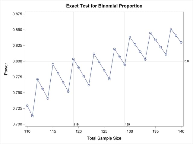
Note the sawtooth pattern in Output 70.2.3. Although the power surpasses the target level of 0.8 at =119, it decreases to 0.79 with =120 and further to 0.76 with =122 before rising again to 0.81 with =123. Not until =130 does the power stay above the 0.8 target. Thus, a more conservative sample size recommendation of 130 might be appropriate, depending on the precise goals of the sample size determination.
In addition to considering alternative sample sizes, you might also want to assess the sensitivity of the power to inaccuracies in assumptions about the true proportion. The following statements produce a plot including true proportion values of 0.18 and 0.22. They are identical to the previous statements except for the additional true proportion values specified with the PROPORTION= option in the ONESAMPLEFREQ statement.
proc power plotonly;
   onesamplefreq test=exact
      sides          = 1
      alpha          = 0.05
      nullproportion = 0.3
      proportion     = 0.18 0.2 0.22
      ntotal         = 119
      power          = .;
   plot x=n min=110 max=140 step=1
      yopts=(ref=.8) xopts=(ref=119 129);
run;
Output 70.2.4 shows the resulting plot.
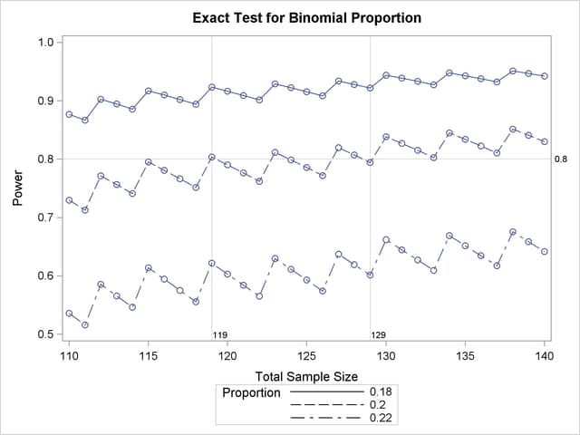
The plot reveals a dramatic sensitivity to the true proportion value. For =119, the power is about 0.92 if the true proportion is 0.18, and as low as 0.62 if the proportion is 0.22. Note also that the power jumps occur at the same sample sizes in all three curves; the curves are only shifted and stretched vertically. This is because spikes and valleys in power curves are invariant to the true proportion value; they are due to changes in the critical value of the test.
A closer look at some ancillary output from the analysis sheds light on this property of the sawtooth pattern. You can add an ODS OUTPUT statement to save the plot content corresponding to Output 70.2.3 to a data set:
proc power plotonly;
   ods output plotcontent=PlotData;
   onesamplefreq test=exact
      sides          = 1
      alpha          = 0.05
      nullproportion = 0.3
      proportion     = 0.2
      ntotal         = 119
      power          = .;
   plot x=n min=110 max=140 step=1
      yopts=(ref=.8) xopts=(ref=119 129);
run;
The PlotData data set contains parameter values for each point in the plot. The parameters include underlying characteristics of the putative test. The following statements print the critical value and actual significance level along with sample size and power:
proc print data=PlotData;
   var NTotal LowerCritVal Alpha Power;
run;
Output 70.2.5 shows the plot data.
| Obs | NTotal | LowerCritVal | Alpha | Power |
|---|---|---|---|---|
| 1 | 110 | 24 | 0.0356 | 0.729 |
| 2 | 111 | 24 | 0.0313 | 0.713 |
| 3 | 112 | 25 | 0.0446 | 0.771 |
| 4 | 113 | 25 | 0.0395 | 0.756 |
| 5 | 114 | 25 | 0.0349 | 0.741 |
| 6 | 115 | 26 | 0.0490 | 0.795 |
| 7 | 116 | 26 | 0.0435 | 0.781 |
| 8 | 117 | 26 | 0.0386 | 0.767 |
| 9 | 118 | 26 | 0.0341 | 0.752 |
| 10 | 119 | 27 | 0.0478 | 0.804 |
| 11 | 120 | 27 | 0.0425 | 0.790 |
| 12 | 121 | 27 | 0.0377 | 0.776 |
| 13 | 122 | 27 | 0.0334 | 0.762 |
| 14 | 123 | 28 | 0.0465 | 0.812 |
| 15 | 124 | 28 | 0.0414 | 0.799 |
| 16 | 125 | 28 | 0.0368 | 0.786 |
| 17 | 126 | 28 | 0.0327 | 0.772 |
| 18 | 127 | 29 | 0.0453 | 0.820 |
| 19 | 128 | 29 | 0.0404 | 0.807 |
| 20 | 129 | 29 | 0.0359 | 0.794 |
| 21 | 130 | 30 | 0.0493 | 0.838 |
| 22 | 131 | 30 | 0.0441 | 0.827 |
| 23 | 132 | 30 | 0.0394 | 0.815 |
| 24 | 133 | 30 | 0.0351 | 0.803 |
| 25 | 134 | 31 | 0.0480 | 0.845 |
| 26 | 135 | 31 | 0.0429 | 0.834 |
| 27 | 136 | 31 | 0.0384 | 0.823 |
| 28 | 137 | 31 | 0.0342 | 0.811 |
| 29 | 138 | 32 | 0.0466 | 0.851 |
| 30 | 139 | 32 | 0.0418 | 0.841 |
| 31 | 140 | 32 | 0.0374 | 0.830 |
Note that whenever the critical value changes, the actual jumps up to a value close to the nominal =0.05, and the power also jumps up. Then while the critical value stays constant, the actual and power slowly decrease. The critical value is independent of the true proportion value. So you can achieve a locally maximal power by choosing a sample size corresponding to a spike on the sawtooth curve, and this choice is locally optimal regardless of the unknown value of the true proportion. Locally optimal sample sizes in this case include 115, 119, 123, 127, 130, and 134.
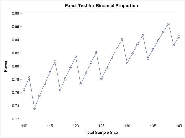
As a point of interest, the power does not always jump sharply and decrease gradually. The shape of the sawtooth depends on the direction of the test and the location of the null proportion relative to 0.5. For example, if the direction of the hypothesis in this example is reversed (by switching true and null proportion values) so that the rejection region is in the upper tail, then the power curve exhibits sharp decreases and gradual increases. The following statements are similar to those producing the plot in Output 70.2.3 but with values of the PROPORTION= and NULLPROPORTION= options switched:
proc power plotonly;
   onesamplefreq test=exact
      sides          = 1
      alpha          = 0.05
      nullproportion = 0.2
      proportion     = 0.3
      ntotal         = 119
      power          = .;
   plot x=n min=110 max=140 step=1;
run;
The resulting plot is shown in Output 70.2.6.
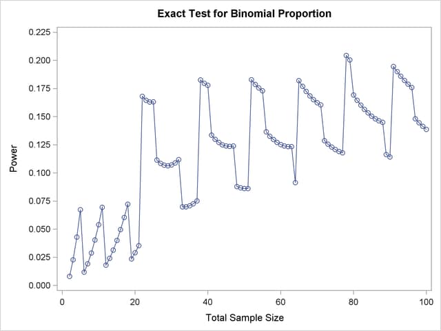
Finally, two-sided tests can lead to even more irregular power curve shapes, since changes in lower and upper critical values affect the power in different ways. The following statements produce a plot of power versus sample size for the scenario of a two-sided test with high alpha and a true proportion close to the null value:
proc power plotonly;
   onesamplefreq test=exact
      sides          = 2
      alpha          = 0.2
      nullproportion = 0.1
      proportion     = 0.09
      ntotal         = 10
      power          = .;
   plot x=n min=2 max=100 step=1;
run;

ods graphics off;
Output 70.2.7 shows the resulting plot.
Due to the irregular shapes of power curves for proportion tests, the question "Which sample size should I use?" is often insufficient. A sample size solution produced directly in PROC POWER reveals the smallest possible sample size to achieve your target power. But as the examples in this section demonstrate, it is helpful to consult graphs for answers to questions such as the following:
Which sample size will guarantee that all higher sample sizes also achieve my target power?
Given a candidate sample size, can I increase it slightly to achieve locally maximal power, or perhaps even decrease it and get higher power?