The PLM Procedure

Example 68.6 Comparing Multiple B-Splines
This example conducts an analysis similar to Example 15 in
,
Examples: GLIMMIX Procedure.
It uses simulated data to perform multiple comparisons among predicted values in a model with group-specific trends that are modeled through regression splines. The estimable functions are formed using nonpositional syntax with constructed effects. Consider the data in the following DATA step. Each of the 100 observations for the continuous response variable y is associated with one of two groups.
data spline;
  input group y @@;
  x = _n_;
  datalines;
 1    -.020 1    0.199 2    -1.36 1    -.026
 2    -.397 1    0.065 2    -.861 1    0.251
 1    0.253 2    -.460 2    0.195 2    -.108
 1    0.379 1    0.971 1    0.712 2    0.811
 2    0.574 2    0.755 1    0.316 2    0.961
 2    1.088 2    0.607 2    0.959 1    0.653
 1    0.629 2    1.237 2    0.734 2    0.299
 2    1.002 2    1.201 1    1.520 1    1.105
 1    1.329 1    1.580 2    1.098 1    1.613
 2    1.052 2    1.108 2    1.257 2    2.005
 2    1.726 2    1.179 2    1.338 1    1.707
 2    2.105 2    1.828 2    1.368 1    2.252
 1    1.984 2    1.867 1    2.771 1    2.052
 2    1.522 2    2.200 1    2.562 1    2.517
 1    2.769 1    2.534 2    1.969 1    2.460
 1    2.873 1    2.678 1    3.135 2    1.705
 1    2.893 1    3.023 1    3.050 2    2.273
 2    2.549 1    2.836 2    2.375 2    1.841
 1    3.727 1    3.806 1    3.269 1    3.533
 1    2.948 2    1.954 2    2.326 2    2.017
 1    3.744 2    2.431 2    2.040 1    3.995
 2    1.996 2    2.028 2    2.321 2    2.479
 2    2.337 1    4.516 2    2.326 2    2.144
 2    2.474 2    2.221 1    4.867 2    2.453
 1    5.253 2    3.024 2    2.403 1    5.498
;
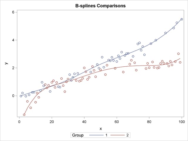
The following statements fit a model with separate trends for the two groups; the trends are modeled as B-splines.
proc orthoreg data=spline;
   class group;
   effect spl = spline(x);
   model y = group spl*group / noint;
   store ortho_spline;
   title 'B-splines Comparisons';
run;
Results from this analysis are shown in Output 68.6.1. The "Parameter Estimates" table shows the estimates for the spline coefficients in the two groups.
| B-splines Comparisons |
| Source | DF | Sum of Squares | Mean Square | F Value | Pr > F |
|---|---|---|---|---|---|
| Model | 13 | 153.0175561 | 11.770581238 | 160.11 | <.0001 |
| Error | 86 | 6.3223804119 | 0.0735160513 | ||
| Corrected Total | 99 | 159.33993651 |
| Root MSE | 0.2711384357 |
|---|---|
| R-Square | 0.9603214326 |
| Parameter | DF | Parameter Estimate | Standard Error | t Value | Pr > |t| |
|---|---|---|---|---|---|
| (group='1') | 1 | 9.70265463962039 | 3.1341899987 | 3.10 | 0.0026 |
| (group='2') | 1 | 6.30619220563569 | 2.6299147768 | 2.40 | 0.0187 |
| spl*group 1 1 | 1 | -11.1786451718041 | 3.7008097395 | -3.02 | 0.0033 |
| spl*group 1 2 | 1 | -20.1946092746139 | 3.9765046236 | -5.08 | <.0001 |
| spl*group 2 1 | 1 | -9.53273697995301 | 3.2575832048 | -2.93 | 0.0044 |
| spl*group 2 2 | 1 | -5.85652496534967 | 2.7906116773 | -2.10 | 0.0388 |
| spl*group 3 1 | 1 | -8.96118371893294 | 3.0717508806 | -2.92 | 0.0045 |
| spl*group 3 2 | 1 | -5.55671605245205 | 2.5716715573 | -2.16 | 0.0335 |
| spl*group 4 1 | 1 | -7.26153231478755 | 3.243690314 | -2.24 | 0.0278 |
| spl*group 4 2 | 1 | -4.36778889738236 | 2.7246809593 | -1.60 | 0.1126 |
| spl*group 5 1 | 1 | -6.44615256510896 | 2.9616955361 | -2.18 | 0.0323 |
| spl*group 5 2 | 1 | -4.03801618914902 | 2.4588839125 | -1.64 | 0.1042 |
| spl*group 6 1 | 1 | -4.63816959094139 | 3.7094636319 | -1.25 | 0.2146 |
| spl*group 6 2 | 1 | -4.30290104395061 | 3.0478540171 | -1.41 | 0.1616 |
| spl*group 7 1 | 0 | 0 | . | . | . |
| spl*group 7 2 | 0 | 0 | . | . | . |
By default, the ORTHOREG procedure constructs B-splines with seven knots. Since B-spline coefficients satisfy a sum-to-one constraint and since the model contains group-specific intercepts, the last spline coefficient for each group is redundant and estimated as 0.
The following statements make a prediction for the input data set by using the SCORE statement with PROC PLM and graph the observed and predicted values in the two groups:
proc plm source=ortho_spline;
   score data=spline out=ortho_pred predicted=p;
run;

proc sgplot data=ortho_pred;
   series  y=p x=x / group=group name="fit";
   scatter y=y x=x / group=group;
   keylegend "fit" / title="Group";
run;
The prediction plot in Output 68.6.2 suggests that there is some separation of the group trends for small values of x and for values that exceed about  .
.
In order to determine the range on which the trends separate significantly, the PLM procedure is executed in the following statements with an ESTIMATE statement that applies group comparisons at a number of values for the spline variable x:
%macro GroupDiff;
   %do x=0 %to 75 %by 5;
      "Diff at x=&x" group 1 -1 group*spl [1,1  &x] [-1,2  &x],
   %end;
   'Diff at x=80' group 1 -1 group*spl [1,1 80] [-1,2 80]
%mend;

proc plm source=ortho_spline;
   show effects;
   estimate %GroupDiff / adjust=simulate seed=1 stepdown;
run;
For example, the following ESTIMATE statement compares the trends between the two groups at  :
:
estimate 'Diff at x=25' group 1 -1 group*spl [1,1 25] [-1,2 25];
The nonpositional syntax is used for the group*spl effect. For example, the specification  requests that the spline be computed at for the second level of variable group. The resulting coefficients are added to the
  vector for the estimate after being multiplied with
  .
.
Because comparisons are made at a large number of values for x, a multiplicity correction is in order to adjust the p-values to reflect familywise error control. Simulated p-values with step-down adjustment are used here.
Output 68.6.3 displays the "Store Information" for the item store and information about the spline effect (the result of the SHOW statement).
| B-splines Comparisons |
| Store Information | |
|---|---|
| Item Store | WORK.ORTHO_SPLINE |
| Data Set Created From | WORK.SPLINE |
| Created By | PROC ORTHOREG |
| Date Created | 18FEB11:10:49:41 |
| Response Variable | y |
| Class Variable | group |
| Constructed Effect | spl |
| Model Effects | group spl*group |
| B-splines Comparisons |
| Knots for Spline Effect spl | ||
|---|---|---|
| Knot Number | Boundary | x |
| 1 | * | -48.50000 |
| 2 | * | -23.75000 |
| 3 | * | 1.00000 |
| 4 | 25.75000 | |
| 5 | 50.50000 | |
| 6 | 75.25000 | |
| 7 | * | 100.00000 |
| 8 | * | 124.75000 |
| 9 | * | 149.50000 |
| B-splines Comparisons |
| Basis Details for Spline Effect spl | |||
|---|---|---|---|
| Column | Support | Support Knots | |
| 1 | -48.50000 | 25.75000 | 1-4 |
| 2 | -48.50000 | 50.50000 | 1-5 |
| 3 | -23.75000 | 75.25000 | 2-6 |
| 4 | 1.00000 | 100.00000 | 3-7 |
| 5 | 25.75000 | 124.75000 | 4-8 |
| 6 | 50.50000 | 149.50000 | 5-9 |
| 7 | 75.25000 | 149.50000 | 6-9 |
Output 68.6.4 displays the results from the ESTIMATE statement.
| Estimates Adjustment for Multiplicity: Holm-Simulated |
||||||
|---|---|---|---|---|---|---|
| Label | Estimate | Standard Error | DF | t Value | Pr > |t| | Adj P |
| Diff at x=0 | 12.4124 | 4.2130 | 86 | 2.95 | 0.0041 | 0.0206 |
| Diff at x=5 | 1.0376 | 0.1759 | 86 | 5.90 | <.0001 | <.0001 |
| Diff at x=10 | 0.3778 | 0.1540 | 86 | 2.45 | 0.0162 | 0.0545 |
| Diff at x=15 | 0.05822 | 0.1481 | 86 | 0.39 | 0.6952 | 0.9101 |
| Diff at x=20 | -0.02602 | 0.1243 | 86 | -0.21 | 0.8346 | 0.9565 |
| Diff at x=25 | 0.02014 | 0.1312 | 86 | 0.15 | 0.8783 | 0.9565 |
| Diff at x=30 | 0.1023 | 0.1378 | 86 | 0.74 | 0.4600 | 0.7418 |
| Diff at x=35 | 0.1924 | 0.1236 | 86 | 1.56 | 0.1231 | 0.2925 |
| Diff at x=40 | 0.2883 | 0.1114 | 86 | 2.59 | 0.0113 | 0.0450 |
| Diff at x=45 | 0.3877 | 0.1195 | 86 | 3.24 | 0.0017 | 0.0096 |
| Diff at x=50 | 0.4885 | 0.1308 | 86 | 3.74 | 0.0003 | 0.0024 |
| Diff at x=55 | 0.5903 | 0.1231 | 86 | 4.79 | <.0001 | <.0001 |
| Diff at x=60 | 0.7031 | 0.1125 | 86 | 6.25 | <.0001 | <.0001 |
| Diff at x=65 | 0.8401 | 0.1203 | 86 | 6.99 | <.0001 | <.0001 |
| Diff at x=70 | 1.0147 | 0.1348 | 86 | 7.52 | <.0001 | <.0001 |
| Diff at x=75 | 1.2400 | 0.1326 | 86 | 9.35 | <.0001 | <.0001 |
| Diff at x=80 | 1.5237 | 0.1281 | 86 | 11.89 | <.0001 | <.0001 |
Notice that the "Store Information" in Output 68.6.3 displays the classification variables (from the CLASS statement in PROC ORTHOREG), the constructed effects (from the EFFECT statement in PROC ORTHOREG), and the model effects (from the MODEL statement in PROC ORTHOREG). Output 68.6.4 shows that at the 5% significance level the trends are significantly different for  and for
  . Between those values you cannot reject the hypothesis of trend congruity.
To see this effect more clearly, you can filter the results by adding the following filtering statement to the previous PROC PLM run:
filter adjp > 0.05;
This produces Output 68.6.5, which displays the subset of the results in Output 68.6.4 that meets the condition in the FILTER expression.
| B-splines Comparisons |
| Estimates Adjustment for Multiplicity: Holm-Simulated |
||||||
|---|---|---|---|---|---|---|
| Label | Estimate | Standard Error | DF | t Value | Pr > |t| | Adj P |
| Diff at x=10 | 0.3778 | 0.1540 | 86 | 2.45 | 0.0162 | 0.0545 |
| Diff at x=15 | 0.05822 | 0.1481 | 86 | 0.39 | 0.6952 | 0.9101 |
| Diff at x=20 | -0.02602 | 0.1243 | 86 | -0.21 | 0.8346 | 0.9565 |
| Diff at x=25 | 0.02014 | 0.1312 | 86 | 0.15 | 0.8783 | 0.9565 |
| Diff at x=30 | 0.1023 | 0.1378 | 86 | 0.74 | 0.4600 | 0.7418 |
| Diff at x=35 | 0.1924 | 0.1236 | 86 | 1.56 | 0.1231 | 0.2925 |