The LOESS Procedure

Example 52.2 Sulfate Deposits in the U.S. for 1990

The following data set contains measurements in grams per square meter of sulfate () deposits during 1990 at 179 sites throughout the 48 contiguous states.

data SO4;
   input Latitude Longitude SO4 @@;
   format Latitude f4.0;
   format Longitude f4.0;
   format SO4 f4.1;
datalines;
32.45833  87.24222 1.403 34.28778  85.96889 2.103
33.07139 109.86472 0.299 36.07167 112.15500 0.304
31.95056 112.80000 0.263 33.60500  92.09722 1.950

   ... more lines ...   

43.87333 104.19222 0.306 44.91722 110.42028 0.210
45.07611  72.67556 2.646
;

As longitudes decrease from west to east in the western hemisphere, the roles of east and west get interchanged if you use these longitudes on the horizontal axis of a plot. You can address this by using negative values to represent longitudes in the western hemisphere. The following statements change the sign of longitude in the SO4 data set and define a format to display these negative values with a suffix of "W".

proc format;
   picture latitude  -90 - 0  = '000S'
                      0  - 90 = '000N';
   picture longitude -180  - 0    = '000W'
                      0    - 180  = '000E';
run;
data SO4;
  set SO4;
  format longitude longitude. latitude  latitude.; 
  longitude = -longitude;
run;

The following statements use ODS Graphics to plot the locations of the sulfate measurements. The circles indicating the locations are colored using a gradient that denotes the value of SO4.

proc template;
   define statgraph gradientScatter;
      beginGraph;
         layout overlay;
            scatterPlot x=longitude y=latitude /
               markercolorgradient = SO4
               markerattrs         = (symbol=circleFilled)
               colormodel          =  ThreeColorRamp
               name                =  "Scatter";   
            scatterPlot x=longitude y=latitude /
               markerattrs         = (symbol=circle);         
            continuousLegend "Scatter"/title= "SO4";
         endlayout;
      endgraph;
   end;
run;

proc sgrender data=SO4 template=gradientScatter;run;

Output 52.2.1 Sulfate Measurements

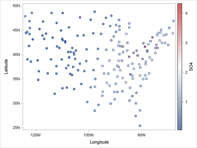
Figure 52.2.1 shows that the largest concentrations of sulfate deposits occur in the northeastern United States.

The following statements fit a loess model.

 
ods graphics on; 

proc loess data=SO4;
   model SO4=Longitude Latitude / degree=2 interp=cubic;
run; 

ods graphics off;

Output 52.2.2 Fit Plot for the SO4 Data

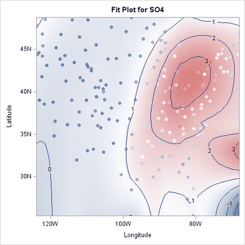
Figure 52.2.2 shows a contour plot of the fitted loess surface overlaid with a scatter plot of the data. The data are colored by the observed sulfate concentrations, using the same color gradient as the gradient-filled contour plot of the fitted surface. Note that for observations where the residual is small, the observations blend in with the contour plot. The greater the size of the residual, the greater the contrast between the observation color and the surface color.

The sulfate measurements are irregularly spaced. To facilitate producing a plot of the fitted loess surface, you can create a data set containing a regular grid of longitudes and latitudes and then use the SCORE statement to evaluate the loess surface at these points. The following statements show how you do this:

 
data PredPoints; 
  format longitude longitude.
         latitude  latitude.; 
   do Latitude = 26 to 46 by 1;
      do Longitude = -79 to -123 by -1;
         output;
      end;
   end;
run;
 
proc loess data=SO4;
   model SO4=Longitude Latitude;
   score data=PredPoints / print;
   ods Output ScoreResults=ScoreOut;
run; 

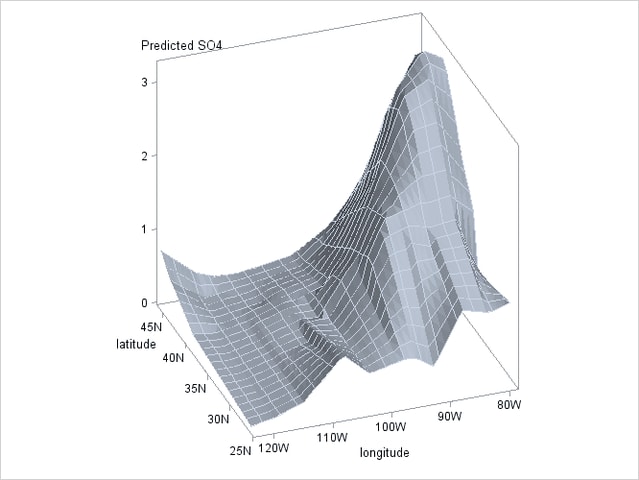
The PRINT option in the SCORE statement requests that the "Score Results" table be displayed as part of the PROC LOESS output. The ODS OUTPUT statement outputs this table to a data set named ScoreOut. If you do not want to display the score results but you do want the score results in an output data set, then you can omit the PRINT option from the SCORE statement. To plot the surface shown in Figure 52.2.3 by using ODS Graphics, use the following statements:

proc template;  
   define statgraph surface;
      begingraph;
         layout overlay3d / rotate=340 tilt=30 cube=false;
            surfaceplotparm x=Longitude y=Latitude z=p_SO4;
         endlayout;
      endgraph;
   end;
run;

proc sgrender data=ScoreOut template=surface;
run;

Output 52.2.3 Loess Fit of SO4 Surface