The HPMIXED Procedure

Model Assumptions

The following sections provide an overview of the approach used by the HPMIXED procedure for likelihood-based analysis of linear mixed models with sparse matrix technique. Additional theory and examples are provided in Littell et al. (1996), Verbeke and Molenberghs (1997, 2000), and Brown and Prescott (1999).

The HPMIXED procedure fits models generally of the form

$\text{[math]}$

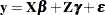Models of this form contain both fixed-effects parameters, $\text{[math]}$ , and random-effects parameters, $\text{[math]}$ ; hence, they are called mixed models. Refer to Henderson (1990) and Searle, Casella, and McCulloch (1992) for historical developments of the mixed model. Note that the matrix $\text{[math]}$ can contain either continuous or dummy variables, just like $\text{[math]}$ .

So far this is the same general form of model fit by the MIXED procedure. The difference between the models handled by the two procedures lies in the assumptions about the distributions of $\text{[math]}$ and $\text{[math]}$ . For both procedures a key assumption is that $\text{[math]}$ and $\text{[math]}$ are normally distributed with

	$\text{[math]}$	$\text{[math]}$	$\text{[math]}$
	$\text{[math]}$	$\text{[math]}$	$\text{[math]}$

The two procedures differ in their assumptions about the variance matrices $\text{[math]}$ and $\text{[math]}$ for $\text{[math]}$ and $\text{[math]}$ , respectively. The MIXED procedure allows a variety of different structures for both $\text{[math]}$ and $\text{[math]}$ ; while in HPMIXED procedure, $\text{[math]}$ is always assumed to be of the form $\text{[math]}$ , and the structures available for modeling $\text{[math]}$ are only a small subset of the structures offered by the MIXED procedure.

Estimates of fixed effects and predictions for random effects are obtained by solving the so-called mixed model equations:

$\text{[math]}$

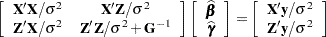Let $\text{[math]}$ denote the coefficient matrix of the mixed model equations:

$\text{[math]}$

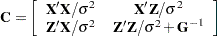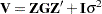Under the assumptions given previously for the moments of $\text{[math]}$ and $\text{[math]}$ , the variance of $\text{[math]}$ is $\text{[math]}$ . You can model $\text{[math]}$ by setting up the random-effects design matrix $\text{[math]}$ and by specifying covariance structures for $\text{[math]}$ . Let $\text{[math]}$ be a vector of all unknown parameters in $\text{[math]}$ . Then the general form of the restricted likelihood function for the mixed models that the HPMIXED procedure can fit is

$\text{[math]}$

where

$\text{[math]}$

and $\text{[math]}$ is the rank of $\text{[math]}$ . The HPMIXED procedure minimizes $\text{[math]}$ over all unknown parameters in $\text{[math]}$ and $\text{[math]}$ by using nonlinear optimization algorithms.