The GENMOD Procedure
-
Overview

-
Getting Started
-
Syntax
PROC GENMOD Statement ASSESS Statement BAYES Statement BY Statement CLASS Statement CONTRAST Statement DEVIANCE Statement EFFECTPLOT Statement ESTIMATE Statement EXACT Statement EXACTOPTIONS Statement FREQ Statement FWDLINK Statement INVLINK Statement LSMEANS Statement LSMESTIMATE Statement MODEL Statement OUTPUT Statement Programming Statements REPEATED Statement SLICE Statement STORE Statement STRATA Statement VARIANCE Statement WEIGHT Statement ZEROMODEL Statement
-
Details
Generalized Linear Models Theory Specification of Effects Parameterization Used in PROC GENMOD Type 1 Analysis Type 3 Analysis Confidence Intervals for Parameters F Statistics Lagrange Multiplier Statistics Predicted Values of the Mean Residuals Multinomial Models Zero-Inflated Models Generalized Estimating Equations Assessment of Models Based on Aggregates of Residuals Case Deletion Diagnostic Statistics Bayesian Analysis Exact Logistic and Exact Poisson Regression Missing Values Displayed Output for Classical Analysis Displayed Output for Bayesian Analysis Displayed Output for Exact Analysis ODS Table Names ODS Graphics
-
Examples
Logistic Regression Normal Regression, Log Link Gamma Distribution Applied to Life Data Ordinal Model for Multinomial Data GEE for Binary Data with Logit Link Function Log Odds Ratios and the ALR Algorithm Log-Linear Model for Count Data Model Assessment of Multiple Regression Using Aggregates of Residuals Assessment of a Marginal Model for Dependent Data Bayesian Analysis of a Poisson Regression Model Exact Poisson Regression
- References
Example 39.10 Bayesian Analysis of a Poisson Regression Model
This example illustrates a Bayesian analysis of a log-linear Poisson regression model. Consider the following data on patients from clinical trials. The data set is a subset of the data described in Ibrahim, Chen, and Lipsitz (1999).
data Liver;
   input X1-X6 Y;
   datalines;
19.1358    50.0110     51.000      0        0       1        3
23.5970    18.4959      3.429      0        0       1        9
20.0474    56.7699      3.429      1        1       0        6
28.0277    59.7836      4.000      0        0       1        6
28.6851    74.1589      5.714      1        0       1        1
18.8092    31.0630      2.286      0        1       1       61
28.7201    52.9178     37.286      1        0       1        6
21.3669    61.6603     54.143      0        1       1        6
23.7332    42.2904      0.571      1        0       1       21

   ... more lines ...

17.0993    48.8384      3.000      0        0       0       9
19.1327    65.3425      2.571      1        0       0       1
17.3010    51.4493      4.429      1        0       0       6
;
The primary interest is in prediction of the number of cancerous liver nodes when a patient enters the trials, by using six other baseline characteristics. The number of nodes is modeled by a Poisson regression model with the six baseline characteristics as covariates. The response and regression variables are as follows:
Y |
Number of Cancerous Liver Nodes |
X1 |
Body Mass Index |
X2 |
Age, in Years |
X3 |
Time Since Diagnosis of Disease, in Weeks |
X4 |
Two Biochemical Markers (each classified as normal=1 or abnormal=0) |
X5 |
Anti Hepatitis B Antigen |
X6 |
Associated Jaundice (yes=1, no=0) |
Two analyses are performed using PROC GENMOD. The first analysis uses noninformative normal prior distributions, and the second analysis uses an informative normal prior for one of the regression parameters.
In the following BAYES statement, COEFFPRIOR=NORMAL specifies a noninformative independent normal prior distribution with zero mean and variance  for each parameter.
The initial analysis is performed using PROC GENMOD to obtain Bayesian estimates of the regression coefficients by using the following SAS statements:
ods graphics on;
proc genmod data=Liver;
   model Y = X1-X6 / dist=Poisson link=log;
   bayes seed=1 coeffprior=normal;
run;
Maximum likelihood estimates of the model parameters are computed by default. These are shown in the "Analysis of Maximum Likelihood Parameter Estimates" table in Output 39.10.1.
| Analysis Of Maximum Likelihood Parameter Estimates | |||||
|---|---|---|---|---|---|
| Parameter | DF | Estimate | Standard Error | Wald 95% Confidence Limits | |
| Intercept | 1 | 2.4508 | 0.2284 | 2.0032 | 2.8984 |
| X1 | 1 | -0.0044 | 0.0080 | -0.0201 | 0.0114 |
| X2 | 1 | -0.0135 | 0.0024 | -0.0181 | -0.0088 |
| X3 | 1 | -0.0029 | 0.0022 | -0.0072 | 0.0014 |
| X4 | 1 | -0.2715 | 0.0795 | -0.4272 | -0.1157 |
| X5 | 1 | 0.3215 | 0.0832 | 0.1585 | 0.4845 |
| X6 | 1 | 0.2077 | 0.0827 | 0.0456 | 0.3698 |
| Scale | 0 | 1.0000 | 0.0000 | 1.0000 | 1.0000 |
| Note: | The scale parameter was held fixed. |
Noninformative independent normal prior distributions with zero means and variances of were used in the initial analysis. These are shown in Output 39.10.2.
| Independent Normal Prior for Regression Coefficients |
||
|---|---|---|
| Parameter | Mean | Precision |
| Intercept | 0 | 1E-6 |
| X1 | 0 | 1E-6 |
| X2 | 0 | 1E-6 |
| X3 | 0 | 1E-6 |
| X4 | 0 | 1E-6 |
| X5 | 0 | 1E-6 |
| X6 | 0 | 1E-6 |
| Initial Values of the Chain | ||||||||
|---|---|---|---|---|---|---|---|---|
| Chain | Seed | Intercept | X1 | X2 | X3 | X4 | X5 | X6 |
| 1 | 1 | 2.450813 | -0.00435 | -0.01347 | -0.00291 | -0.27149 | 0.321507 | 0.207713 |
Summary statistics for the posterior sample are displayed in the "Fit Statistics," "Descriptive Statistics for the Posterior Sample," "Interval Statistics for the Posterior Sample," and "Posterior Correlation Matrix" tables in Output 39.10.4, Output 39.10.5, Output 39.10.6, and Output 39.10.7, respectively. Since noninformative prior distributions for the regression coefficients were used, the mean and standard deviations of the posterior distributions for the model parameters are close to the maximum likelihood estimates and standard errors.
| Fit Statistics | |
|---|---|
| DIC (smaller is better) | 829.729 |
| pD (effective number of parameters) | 6.966 |
| Posterior Summaries | ||||||
|---|---|---|---|---|---|---|
| Parameter | N | Mean | Standard Deviation |
Percentiles | ||
| 25% | 50% | 75% | ||||
| Intercept | 10000 | 2.4520 | 0.2268 | 2.2997 | 2.4521 | 2.6053 |
| X1 | 10000 | -0.00473 | 0.00801 | -0.0100 | -0.00465 | 0.000759 |
| X2 | 10000 | -0.0134 | 0.00236 | -0.0150 | -0.0134 | -0.0118 |
| X3 | 10000 | -0.00309 | 0.00220 | -0.00455 | -0.00305 | -0.00158 |
| X4 | 10000 | -0.2705 | 0.0792 | -0.3241 | -0.2697 | -0.2172 |
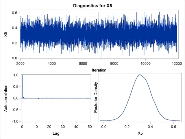
| X5 | 10000 | 0.3193 | 0.0834 | 0.2629 | 0.3180 | 0.3762 |
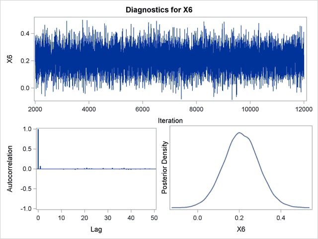
| X6 | 10000 | 0.2095 | 0.0834 | 0.1538 | 0.2086 | 0.2653 |
| Posterior Intervals | |||||
|---|---|---|---|---|---|
| Parameter | Alpha | Equal-Tail Interval | HPD Interval | ||
| Intercept | 0.050 | 2.0169 | 2.9056 | 2.0069 | 2.8923 |
| X1 | 0.050 | -0.0210 | 0.0106 | -0.0212 | 0.0103 |
| X2 | 0.050 | -0.0181 | -0.00878 | -0.0181 | -0.00885 |
| X3 | 0.050 | -0.00757 | 0.00109 | -0.00764 | 0.000989 |
| X4 | 0.050 | -0.4250 | -0.1132 | -0.4232 | -0.1119 |
| X5 | 0.050 | 0.1552 | 0.4821 | 0.1647 | 0.4905 |
| X6 | 0.050 | 0.0477 | 0.3749 | 0.0490 | 0.3758 |
| Posterior Correlation Matrix | |||||||
|---|---|---|---|---|---|---|---|
| Parameter | Intercept | X1 | X2 | X3 | X4 | X5 | X6 |
| Intercept | 1.000 | -0.705 | -0.430 | -0.046 | -0.225 | -0.180 | -0.415 |
| X1 | -0.705 | 1.000 | -0.211 | -0.013 | -0.068 | 0.067 | 0.128 |
| X2 | -0.430 | -0.211 | 1.000 | -0.006 | 0.070 | 0.057 | 0.118 |
| X3 | -0.046 | -0.013 | -0.006 | 1.000 | 0.016 | -0.055 | -0.089 |
| X4 | -0.225 | -0.068 | 0.070 | 0.016 | 1.000 | -0.011 | 0.089 |
| X5 | -0.180 | 0.067 | 0.057 | -0.055 | -0.011 | 1.000 | -0.042 |
| X6 | -0.415 | 0.128 | 0.118 | -0.089 | 0.089 | -0.042 | 1.000 |
Posterior sample autocorrelations for each model parameter are shown in Output 39.10.8. The autocorrelation after 10 lags is negligible for all parameters, indicating good mixing in the Markov chain.
| Posterior Autocorrelations | ||||
|---|---|---|---|---|
| Parameter | Lag 1 | Lag 5 | Lag 10 | Lag 50 |
| Intercept | 0.0551 | -0.0134 | -0.0101 | 0.0012 |
| X1 | 0.0894 | -0.0054 | -0.0080 | 0.0019 |
| X2 | 0.1197 | -0.0170 | 0.0061 | 0.0006 |
| X3 | 0.0324 | -0.0036 | -0.0033 | -0.0160 |
| X4 | 0.0309 | 0.0056 | 0.0053 | 0.0115 |
| X5 | 0.0402 | 0.0015 | -0.0111 | 0.0123 |
| X6 | 0.0696 | -0.0047 | -0.0024 | 0.0006 |
The p-values for the Geweke test statistics shown in Output 39.10.9 all indicate convergence of the MCMC. See the section Assessing Markov Chain Convergence for more information about convergence diagnostics and their interpretation.
| Geweke Diagnostics | ||
|---|---|---|
| Parameter | z | Pr > |z| |
| Intercept | 0.9855 | 0.3244 |
| X1 | -1.0835 | 0.2786 |
| X2 | -0.3847 | 0.7005 |
| X3 | 0.6715 | 0.5019 |
| X4 | 0.1328 | 0.8943 |
| X5 | 1.0698 | 0.2847 |
| X6 | -0.1647 | 0.8692 |
The effective sample sizes for each parameter are shown in Output 39.10.10.
| Effective Sample Sizes | |||
|---|---|---|---|
| Parameter | ESS | Autocorrelation Time |
Efficiency |
| Intercept | 9245.8 | 1.0816 | 0.9246 |
| X1 | 8179.5 | 1.2226 | 0.8179 |
| X2 | 8067.8 | 1.2395 | 0.8068 |
| X3 | 9390.6 | 1.0649 | 0.9391 |
| X4 | 9157.6 | 1.0920 | 0.9158 |
| X5 | 9665.2 | 1.0346 | 0.9665 |
| X6 | 8778.7 | 1.1391 | 0.8779 |
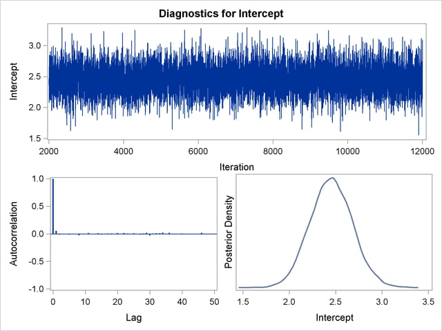
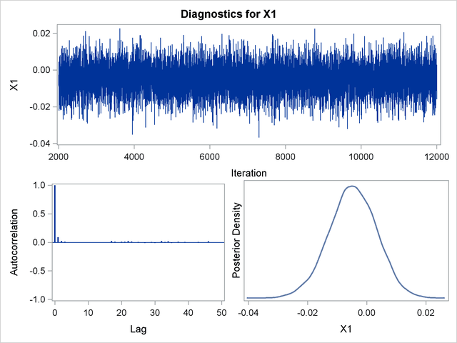
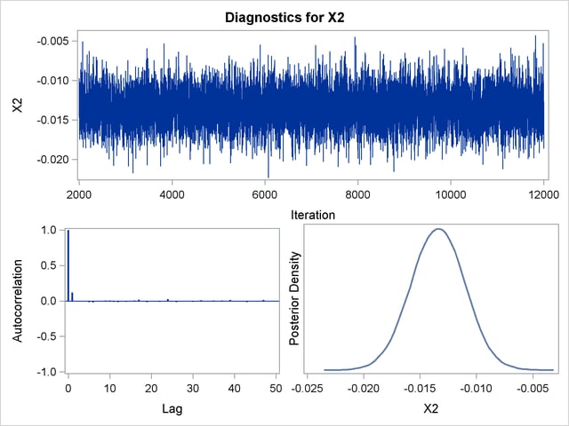
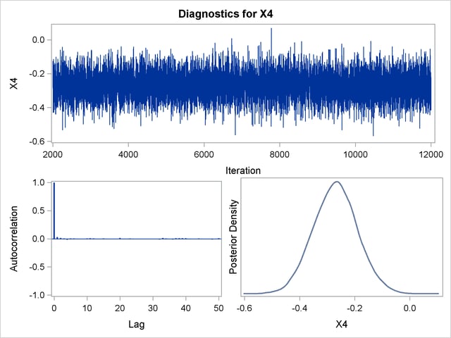
Trace, autocorrelation, and density plots for the seven model parameters are shown in Output 39.10.11 through Output 39.10.17. All indicate satisfactory convergence of the Markov chain.

In order to illustrate the use of an informative prior distribution, suppose that researchers expect that a unit increase in body mass index (X1) will be associated with an increase in the mean number of nodes of between 10% and 20%, and they want to incorporate this prior knowledge in the Bayesian analysis. For log-linear models, the mean and linear predictor are related by  . If
. If  and
and  are two values of body mass index,
  and
and  are the two mean values, and all other covariates remain equal for the two values of X1, then
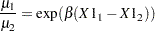 |
so that for a unit change in X1,
 |
If  , then
 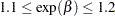 , or
, or  . This gives you guidance in specifying a prior distribution for the
  for body mass index. Taking the mean of the prior normal distribution to be the midrange of the values of , and taking
  to be the extremes of the range, an
  is the resulting prior distribution. The second analysis uses this informative normal prior distribution for the coefficient of
  and uses independent noninformative normal priors with zero means and variances equal to for the remaining model regression parameters.
In the following BAYES statement, COEFFPRIOR=NORMAL(INPUT=NormalPrior) specifies the normal prior distribution for the regression coefficients with means and variances contained in the data set NormalPrior.
An analysis is performed using PROC GENMOD to obtain Bayesian estimates of the regression coefficients by using the following SAS statements:
data NormalPrior;
  input _type_ $ Intercept X1-X6;
  datalines;
Var  1e6   0.0005      1e6      1e6      1e6      1e6      1e6
Mean 0.0   0.1385      0.0      0.0      0.0      0.0      0.0
;
proc genmod data=Liver;
   model Y = X1-X6 / dist=Poisson link=log;
   bayes seed=1 plots=none coeffprior=normal(input=NormalPrior) ;
run;
ods graphics off;
The prior distributions for the regression parameters are shown in Output 39.10.18.
| Independent Normal Prior for Regression Coefficients |
||
|---|---|---|
| Parameter | Mean | Precision |
| Intercept | 0 | 1E-6 |
| X1 | 0.1385 | 2000 |
| X2 | 0 | 1E-6 |
| X3 | 0 | 1E-6 |
| X4 | 0 | 1E-6 |
| X5 | 0 | 1E-6 |
| X6 | 0 | 1E-6 |
| Initial Values of the Chain | ||||||||
|---|---|---|---|---|---|---|---|---|
| Chain | Seed | Intercept | X1 | X2 | X3 | X4 | X5 | X6 |
| 1 | 1 | 2.14282 | 0.010595 | -0.01434 | -0.00301 | -0.28062 | 0.334983 | 0.231213 |
Goodness-of-fit, summary, and interval statistics are shown in Output 39.10.20. Except for X1, the statistics shown in Output 39.10.20 are very similar to the previous statistics for noninformative priors shown in Output 39.10.4 through Output 39.10.7. The point estimate for X1 is now positive. This is expected because the prior distribution on  is quite informative. The distribution reflects the belief that the coefficient is positive. The distribution places the majority of its probability density on positive values. As a result, the posterior density of places more likelihood on positive values than in the noninformative case.
| Fit Statistics | |
|---|---|
| DIC (smaller is better) | 833.134 |
| pD (effective number of parameters) | 6.861 |
| Posterior Summaries | ||||||
|---|---|---|---|---|---|---|
| Parameter | N | Mean | Standard Deviation |
Percentiles | ||
| 25% | 50% | 75% | ||||
| Intercept | 10000 | 2.1393 | 0.2160 | 1.9929 | 2.1417 | 2.2845 |
| X1 | 10000 | 0.0104 | 0.00685 | 0.00583 | 0.0106 | 0.0151 |
| X2 | 10000 | -0.0143 | 0.00236 | -0.0159 | -0.0143 | -0.0127 |
| X3 | 10000 | -0.00318 | 0.00218 | -0.00463 | -0.00313 | -0.00170 |
| X4 | 10000 | -0.2801 | 0.0798 | -0.3342 | -0.2807 | -0.2258 |
| X5 | 10000 | 0.3336 | 0.0834 | 0.2772 | 0.3337 | 0.3902 |
| X6 | 10000 | 0.2333 | 0.0822 | 0.1791 | 0.2327 | 0.2892 |
| Posterior Intervals | |||||
|---|---|---|---|---|---|
| Parameter | Alpha | Equal-Tail Interval | HPD Interval | ||
| Intercept | 0.050 | 1.7161 | 2.5599 | 1.7075 | 2.5507 |
| X1 | 0.050 | -0.00323 | 0.0236 | -0.00264 | 0.0241 |
| X2 | 0.050 | -0.0189 | -0.00960 | -0.0189 | -0.00972 |
| X3 | 0.050 | -0.00754 | 0.00101 | -0.00754 | 0.000963 |
| X4 | 0.050 | -0.4348 | -0.1223 | -0.4311 | -0.1196 |
| X5 | 0.050 | 0.1705 | 0.4970 | 0.1661 | 0.4915 |
| X6 | 0.050 | 0.0696 | 0.3968 | 0.0655 | 0.3904 |