The CATMOD Procedure

Example 29.3 Logistic Regression, Standard Response Function

In this data set, from Cox and Snell (1989), ingots are prepared with different heating and soaking times and tested for their readiness to be rolled. The following DATA step creates a response variable Y with value 1 for ingots that are not ready and value 0 otherwise. The explanatory variables are Heat and Soak.

data ingots;
   input Heat Soak nready ntotal @@;
   Count=nready;
   Y=1;
   output;
   Count=ntotal-nready;
   Y=0;
   output;
   drop nready ntotal;
   datalines;
7 1.0 0 10   14 1.0 0 31   27 1.0 1 56   51 1.0 3 13
7 1.7 0 17   14 1.7 0 43   27 1.7 4 44   51 1.7 0  1
7 2.2 0  7   14 2.2 2 33   27 2.2 0 21   51 2.2 0  1
7 2.8 0 12   14 2.8 0 31   27 2.8 1 22   51 4.0 0  1
7 4.0 0  9   14 4.0 0 19   27 4.0 1 16
;

Logistic regression analysis is often used to investigate the relationship between discrete response variables and continuous explanatory variables. For logistic regression, the continuous design-effects are declared in a DIRECT statement. The following statements produce Output 29.3.1 through Output 29.3.6:

title 'Maximum Likelihood Logistic Regression';
proc catmod data=ingots;
   weight Count;
   direct Heat Soak;
   model Y=Heat Soak / freq covb corrb itprint design;
quit;

You can verify that the populations are defined as you intended by looking at the "Population Profiles" table in Output 29.3.1.

Output 29.3.1 Maximum Likelihood Logistic Regression

Maximum Likelihood Logistic Regression

The CATMOD Procedure

Data Summary
Response	Y	Response Levels	2
Weight Variable	Count	Populations	19
Data Set	INGOTS	Total Frequency	387
Frequency Missing	0	Observations	25

Population Profiles
Sample	Heat	Soak	Sample Size
1	7	1	10
2	7	1.7	17
3	7	2.2	7
4	7	2.8	12
5	7	4	9
6	14	1	31
7	14	1.7	43
8	14	2.2	33
9	14	2.8	31
10	14	4	19
11	27	1	56
12	27	1.7	44
13	27	2.2	21
14	27	2.8	22
15	27	4	16
16	51	1	13
17	51	1.7	1
18	51	2.2	1
19	51	4	1

Since the "Response Profiles" table in Output 29.3.2 shows the response level ordering as 0, 1, the default response function, the logit, is defined as $\text{[math]}$ .

Output 29.3.2 Response Summaries

Response Profiles
Response	Y
1	0
2	1

Response Frequencies
Sample	Response Number
Sample	1	2
1	10	0
2	17	0
3	7	0
4	12	0
5	9	0
6	31	0
7	43	0
8	31	2
9	31	0
10	19	0
11	55	1
12	40	4
13	21	0
14	21	1
15	15	1
16	10	3
17	1	0
18	1	0
19	1	0

The values of the continuous variable are inserted into the design matrix (Output 29.3.3).

Output 29.3.3 Design Matrix

Response Functions and Design Matrix
Sample	Response Function	Design Matrix
Sample	Response Function	1	2	3
1	2.99573	1	7	1
2	3.52636	1	7	1.7
3	2.63906	1	7	2.2
4	3.17805	1	7	2.8
5	2.89037	1	7	4
6	4.12713	1	14	1
7	4.45435	1	14	1.7
8	2.74084	1	14	2.2
9	4.12713	1	14	2.8
10	3.63759	1	14	4
11	4.00733	1	27	1
12	2.30259	1	27	1.7
13	3.73767	1	27	2.2
14	3.04452	1	27	2.8
15	2.70805	1	27	4
16	1.20397	1	51	1
17	0.69315	1	51	1.7
18	0.69315	1	51	2.2
19	0.69315	1	51	4

Seven Newton-Raphson iterations are required to find the maximum likelihood estimates (Output 29.3.4).

Output 29.3.4 Iteration History

Maximum Likelihood Analysis
Iteration	Sub Iteration	-2 Log Likelihood	Convergence Criterion	Parameter Estimates
Iteration	Sub Iteration	-2 Log Likelihood	Convergence Criterion	1	2	3
0	0	536.49592	1.0000	0	0	0
1	0	152.58961	0.7156	2.1594	-0.0139	-0.003733
2	0	106.76066	0.3003	3.5334	-0.0363	-0.0120
3	0	96.692171	0.0943	4.7489	-0.0640	-0.0299
4	0	95.383825	0.0135	5.4138	-0.0790	-0.0498
5	0	95.345659	0.000400	5.5539	-0.0819	-0.0564
6	0	95.345613	4.8289E-7	5.5592	-0.0820	-0.0568
7	0	95.345613	7.728E-13	5.5592	-0.0820	-0.0568

Maximum likelihood computations converged.

The analysis of variance table (Output 29.3.5) shows that the model fits since the likelihood ratio goodness-of-fit test is nonsignificant. It also shows that the length of heating time is a significant factor with respect to readiness but that length of soaking time is not.

Output 29.3.5 Analysis of Variance Table

Maximum Likelihood Analysis of Variance
Source	DF	Chi-Square	Pr > ChiSq
Intercept	1	24.65	<.0001
Heat	1	11.95	0.0005
Soak	1	0.03	0.8639
Likelihood Ratio	16	13.75	0.6171

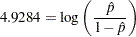
From the table of maximum likelihood estimates in Output 29.3.6, the fitted model is

$\text{[math]}$

For example, for Sample 1 with Heat $\text{[math]}$ and Soak $\text{[math]}$ , the estimate is

$\text{[math]}$

Output 29.3.6 Maximum Likelihood Estimates, Covariances, and Correlations

Analysis of Maximum Likelihood Estimates
Parameter	Estimate	Standard Error	Chi- Square	Pr > ChiSq
Intercept	5.5592	1.1197	24.65	<.0001
Heat	-0.0820	0.0237	11.95	0.0005
Soak	-0.0568	0.3312	0.03	0.8639

Covariance Matrix of the Maximum Likelihood Estimates
Row	Parameter	Col1	Col2	Col3
1	Intercept	1.2537133	-0.0215664	-0.2817648
2	Heat	-0.0215664	0.0005633	0.0026243
3	Soak	-0.2817648	0.0026243	0.1097020

Correlation Matrix of the Maximum Likelihood Estimates
Row	Parameter	Col1	Col2	Col3
1	Intercept	1.00000	-0.81152	-0.75977
2	Heat	-0.81152	1.00000	0.33383
3	Soak	-0.75977	0.33383	1.00000

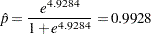
Predicted values of the logits, as well as the probabilities of readiness, could be obtained by specifying PRED=PROB in the MODEL statement. For the example of Sample 1 with Heat $\text{[math]}$ and Soak $\text{[math]}$ , PRED=PROB would give an estimate of the probability of readiness equal to 0.9928 since

$\text{[math]}$

implies that

$\text{[math]}$

As another consideration, since soaking time is nonsignificant, you could fit another model that deleted the variable Soak.