PROC TRANSREG: Simultaneously Fitting Two Regression Functions

The TRANSREG Procedure

Simultaneously Fitting Two Regression Functions

One application of ordinary multiple regression is fitting two or more regression lines through a single scatter plot. With PROC TRANSREG, this application can easily be generalized to fit separate or parallel curves. To illustrate, consider a data set with two groups and a group membership variable g that has the value 1 for one group and 2 for the other group. The data set also has a continuous independent variable x and a continuous dependent variable y. When g is crossed with x, the variables g1x and g2x both have a large partition of zeros. For this reason, the KNOTS= t-option is specified instead of the NKNOTS= t-option. (The latter would put a number of knots in the partition of zeros.) The following example generates an artificial data set with two curves. While these artificial data are clearly not realistic, their distinct pattern helps illustrate how fitting simultaneous regression functions works. The following statements generate data and show how PROC TRANSREG fits lines, curves, and monotone curves through a scatter plot:


title 'Separate Curves, Separate Intercepts';

data a;
   do x = -2 to 3 by 0.025;
      g = 1;
      y = 8*(x*x + 2*cos(x*6)) + 15*normal(7654321);
      output;
      g = 2;
      y = 4*(-x*x + 4*sin(x*4)) - 40 + 15*normal(7654321);
      output;
   end;
run;

ods graphics on;
ods select fitplot(persist);

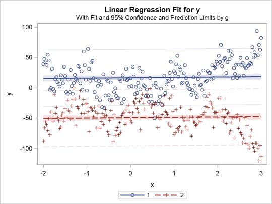
title 'Parallel Lines, Separate Intercepts';

proc transreg data=a solve;
   model identity(y)=class(g) identity(x);
run;

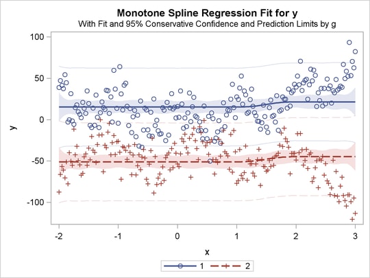
title 'Parallel Monotone Curves, Separate Intercepts';

proc transreg data=a;
   model identity(y)=class(g) mspline(x / knots=-1.5 to 2.5 by 0.5);
run;

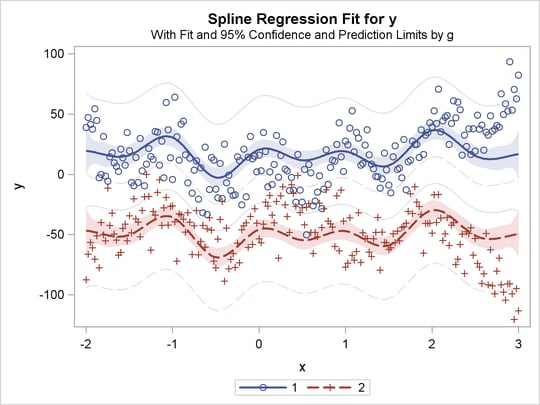
title 'Parallel Curves, Separate Intercepts';

proc transreg data=a solve;
   model identity(y)=class(g) spline(x / knots=-1.5 to 2.5 by 0.5);
run;

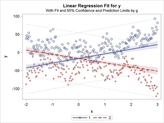
title 'Separate Slopes, Same Intercept';

proc transreg data=a;
   model identity(y)=class(g / zero=none) * identity(x);
run;

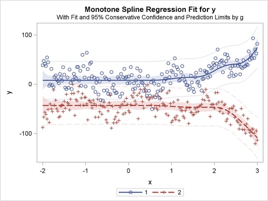
title 'Separate Monotone Curves, Same Intercept';

proc transreg data=a;
   model identity(y) = class(g / zero=none) *
                       mspline(x / knots=-1.5 to 2.5 by 0.5);
run;

title 'Separate Curves, Same Intercept';

proc transreg data=a solve;
   model identity(y) = class(g / zero=none) *
                       spline(x / knots=-1.5 to 2.5 by 0.5);
run;

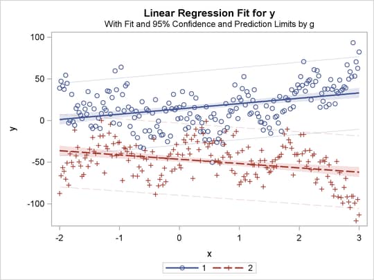
title 'Separate Slopes, Separate Intercepts';

proc transreg data=a;
   model identity(y) = class(g / zero=none) | identity(x);
run;

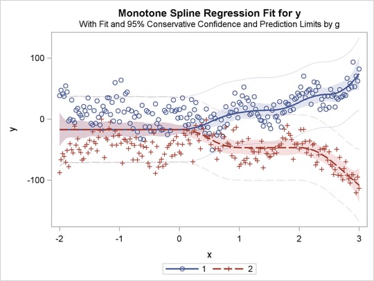
title 'Separate Monotone Curves, Separate Intercepts';

proc transreg data=a;
   model identity(y) = class(g / zero=none) |
                       mspline(x / knots=-1.5 to 2.5 by 0.5);
run;

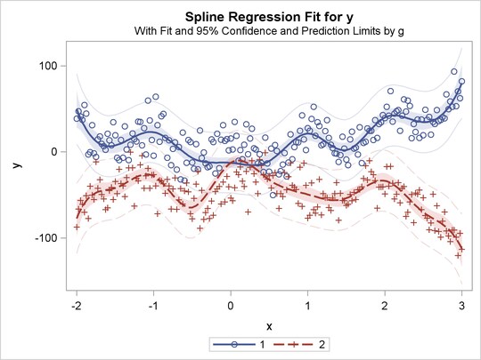
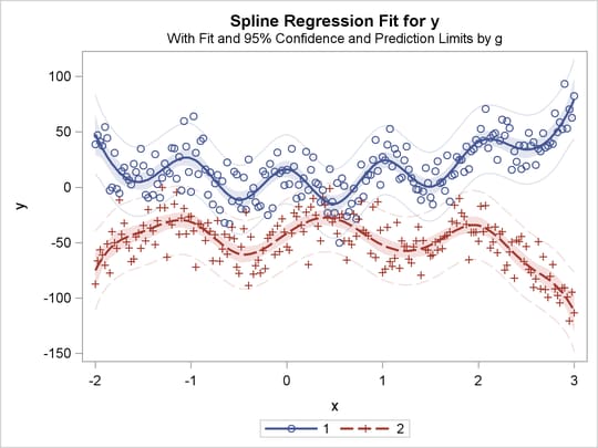
title 'Separate Curves, Separate Intercepts';

proc transreg data=a solve;
   model identity(y) = class(g / zero=none) |
                       spline(x / knots=-1.5 to 2.5 by 0.5);
run;

ods graphics off;
ods select all;

The previous statements produce Figure 91.32 through Figure 91.40. Only the fit plots are generated and displayed.

Figure 91.32 Parallel Lines, Separate Intercepts