Example 76.2 Response Surface Analysis with Covariates

One way of viewing covariates is as extra sources of variation in the dependent variable that can mask the variation due to primary factors. This example demonstrates the use of the COVAR= option in PROC RSREG to fit a response surface model to the dependent variables corrected for the covariates.

You have a chemical process with a yield that you hypothesize to be dependent on three factors: reaction time, reaction temperature, and reaction pressure. You perform an experiment to measure this dependence. You are willing to include up to 20 runs in your experiment, but you can perform no more than 8 runs on the same day, so the design for the experiment is composed of three blocks. Additionally, you know that the grade of raw material for the reaction has a significant impact on the yield. You have no control over this, but you keep track of it. The following statements create a SAS data set containing the results of the experiment:

data Experiment;
   input Day Grade Time Temp Pressure Yield;
   datalines;
1 67      -1     -1     -1         32.98
1 68      -1      1      1         47.04
1 70       1     -1      1         67.11
1 66       1      1     -1         26.94
1 74       0      0      0        103.22
1 68       0      0      0         42.94
2 75      -1     -1      1        122.93
2 69      -1      1     -1         62.97
2 70       1     -1     -1         72.96
2 71       1      1      1         94.93
2 72       0      0      0         93.11
2 74       0      0      0        112.97
3 69       1.633  0      0         78.88
3 67      -1.633  0      0         52.53
3 68       0      1.633  0         68.96
3 71       0     -1.633  0         92.56
3 70       0      0      1.633     88.99
3 72       0      0     -1.633    102.50
3 70       0      0      0         82.84
3 72       0      0      0        103.12
;

Your first analysis neglects to take the covariates into account. The following statements use PROC RSREG to fit a response surface to the observed yield, but note that Day and Grade are omitted:

proc rsreg data=Experiment;
   model Yield = Time Temp Pressure;
run;

The ANOVA results shown in Output 76.2.1 indicate that no process variable effects are significantly larger than the background noise.

However, when the yields are adjusted for covariate effects of day and grade of raw material, very strong process variable effects are revealed. The following statements produce the ANOVA results in Output 76.2.2. Note that in order to include the effects of the classification factor Day as covariates, you need to create dummy variables indicating each day separately.

   data Experiment; 
      set Experiment;
      d1 = (Day = 1);
      d2 = (Day = 2);
      d3 = (Day = 3);

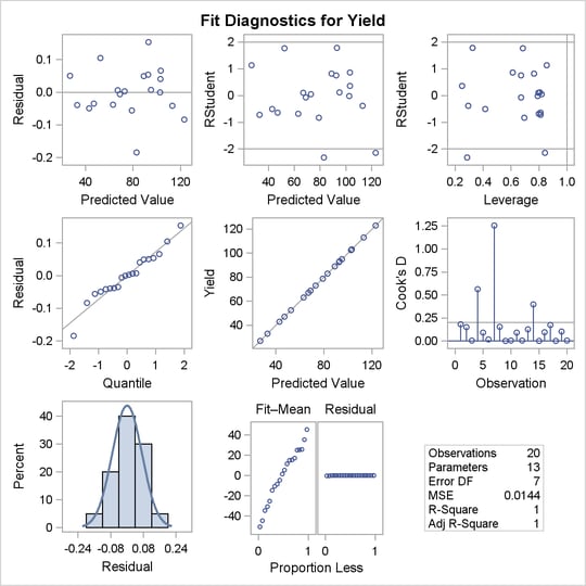
ods graphics on;
proc rsreg data=Experiment plots=all;
   model Yield = d1-d3 Grade Time Temp Pressure / covar=4;
run;
ods graphics off;

The results show very strong effects due to both the covariates and the process variables.

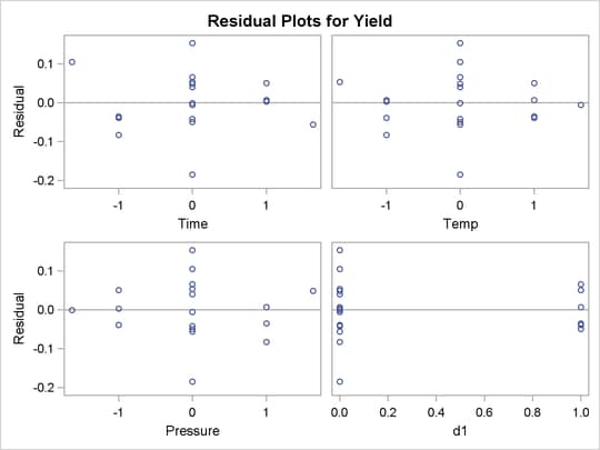
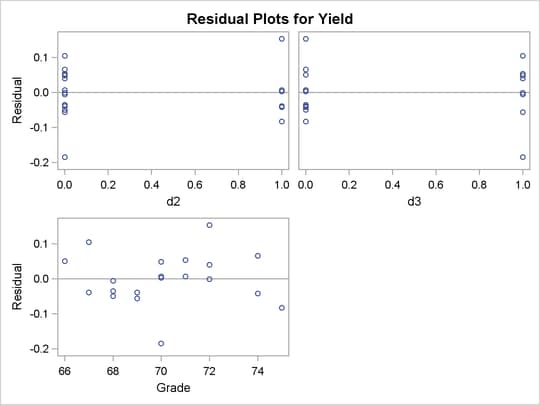
The number of observations in the data set might be too small for the diagnostic plots in Output 76.2.3 to dependably identify problems; however, some outliers are indicated. The residual plots in Output 76.2.4 do not display any obvious structure.

Output 76.2.3 Fit Diagnostics

Output 76.2.4 Residual Plots