| The ROBUSTREG Procedure |
Example 75.5 Robust Diagnostics
This example models the selling price of a house as a function of several covariates. One of these covariates is a classification variable that indicates whether a house is located on a corner lot (called a corner house in this example). Because corner houses are relatively rare, the inclusion of this classification effect in the model introduces a low-dimensional structure (that is, the majority of the observations are located in a lower dimensional hyperplane defined by being non-corner houses) into the design matrix. As discussed in Robust Distance, the presence of this low dimensional structure causes difficulties in the traditional computation of robust distances. This example illustrates how you can use the projected robust distance to address those difficulties and to obtain meaningful leverage diagnostics. It also shows how you can use the RDPLOT and DDPLOT options to illustrate the outlier-leverage relationship.
The following house price data set contains 66 home resale records on seven variables from February 15 to April 30, 1993 (The Data and Story Library, 2005). The records are randomly selected from the database maintained by the Albuquerque Board of Realtors.
    data house;
      input price sqft age feats ne cor tax @@;
      label price = "Selling price"
            sqft  = "Square feet of living space"
            age   = "Age of home in year"
            feats = "Number out of 11 features (dishwasher, refrigerator,
                     microwave, disposer, washer, intercom, skylight(s),
                     compactor, dryer, handicap fit, cable TV access)"
            ne    = "Located in northeast sector of city (1) or not (0)"
            cor   = "Corner location (1) or not (0)"
            tax   = "Annual taxes";
      sum = sqft+age+feats+ne+cor+tax;
      id  = _N_;
      datalines;
       2050 2650 13 7 1 0 1639
       2150 2664  6 5 1 0 1193
       2150 2921  3 6 1 0 1635
       1999 2580  4 4 1 0 1732

   ... more lines ...

        869 1165  7 4 0 0  694
        766 1200  7 4 0 1  634
        739  970  4 4 0 1  541
       ;
       run;
To illustrate the dependence detection ability of the generalized MCD algorithm, an extra variable sum is created such that all the observations satisfy
 |
Adding sum does not change the rank of the original design matrix, so that sum is expected to be ignored in the model and also in the diagnostics. The next statements apply the MM method and the generalized MCD algorithm to the house price data.
 ods graphics on;
 ods trace output notes;
 proc robustreg data=house method=MM plots=all;
    model price= sqft age feats ne cor tax sum/leverage(opc) diagnostics;
 run;
 ods trace off;
As shown in Output 75.5.1 and Output 75.5.2, PROC ROBUSTREG finds the design dependence equation and forces the parameter estimate of variable sum to be zero.
| Parameter Estimates | |||||||
|---|---|---|---|---|---|---|---|
| Parameter | DF | Estimate | Standard Error | 95% Confidence Limits | Chi-Square | Pr > ChiSq | |
| Intercept | 1 | 46.4062 | 79.1714 | -108.767 | 201.5792 | 0.34 | 0.5578 |
| sqft | 1 | 0.3809 | 0.0756 | 0.2327 | 0.5291 | 25.37 | <.0001 |
| age | 1 | -2.6067 | 1.7610 | -6.0582 | 0.8449 | 2.19 | 0.1388 |
| feats | 1 | 8.3627 | 14.7107 | -20.4697 | 37.1951 | 0.32 | 0.5697 |
| ne | 1 | 65.0081 | 40.1329 | -13.6508 | 143.6671 | 2.62 | 0.1053 |
| cor | 1 | -19.2997 | 38.1907 | -94.1520 | 55.5526 | 0.26 | 0.6133 |
| tax | 1 | 0.4699 | 0.1260 | 0.2229 | 0.7170 | 13.90 | 0.0002 |
| sum | 0 | 0.0000 | . | . | . | . | . |
| Scale | 0 | 157.5593 | |||||
Moreover, PROC ROBUSTREG also identifies a robust dependence equation on cor in Output 75.5.3, which holds for  of the observations but not for the entire data set.
Another way to represent the low-dimensional structure is to specify the coefficients of the MCD-dropped components on the data (see Output 75.5.4), which form a basis of the complementary space to the relevant low-dimensional hyperplane.
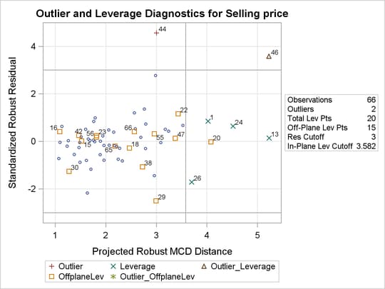
By definitions of projected robust distance and leverage point, an observation is called an off-plane leverage point if at least one of the robust or design dependence equations does not apply to the observation. In this example, the observations with cor  are all off-plane leverage points. Output 75.5.5 lists the leverage points and outliers along with the relevant distance measurements and standardized residuals.
| Diagnostics | ||||||
|---|---|---|---|---|---|---|
| Obs | Projected Distance | Leverage | Standardized Robust Residual |
Outlier | ||
| Mahalanobis | Robust | Off-Plane | ||||
| 1 | 3.5567 | 4.0211 | 0.0000 | * | 0.8522 | |
| 13 | 4.0034 | 5.2310 | 0.0000 | * | 0.1411 | |
| 15 | 1.3221 | 1.5219 | 2.3681 | * | 0.0226 | |
| 16 | 1.0839 | 1.0905 | 2.3681 | * | 0.4148 | |
| 18 | 1.9452 | 2.4655 | 2.3681 | * | -0.2789 | |
| 20 | 3.6006 | 4.0771 | 2.3681 | * | -0.0150 | |
| 22 | 3.0210 | 3.4307 | 2.3681 | * | 1.1664 | |
| 23 | 1.5920 | 1.8197 | 2.3681 | * | 0.2422 | |
| 24 | 3.4967 | 4.5154 | 0.0000 | * | 0.6464 | |
| 26 | 3.0420 | 3.6975 | 0.0000 | * | -1.7068 | |
| 29 | 2.3264 | 2.9925 | 2.3681 | * | -2.4980 | |
| 30 | 1.2587 | 1.2714 | 2.3681 | * | -1.2558 | |
| 38 | 2.4064 | 2.7249 | 2.3681 | * | -1.0620 | |
| 42 | 1.4722 | 1.4645 | 2.3681 | * | 0.2584 | |
| 44 | 2.8491 | 3.0019 | 0.0000 | 4.5665 | * | |
| 46 | 3.9725 | 5.2271 | 0.0000 | * | 3.5835 | * |
| 47 | 2.9431 | 3.3728 | 2.3681 | * | 0.1365 | |
| 55 | 2.2325 | 2.9590 | 2.3681 | * | 0.3217 | |
| 56 | 1.7999 | 1.8119 | 2.3681 | * | 0.1715 | |
| 65 | 1.8831 | 2.1822 | 2.3681 | * | -0.1990 | |
| 66 | 2.2483 | 2.5673 | 2.3681 | * | 0.4134 | |
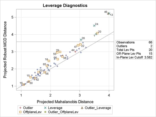
From Output 75.5.6 and Output 75.5.7, you can see that there is no apparent corner-related difference for the houses in terms of standardized robust residual and projected MD versus projected RD, although all the corner houses are defined as off-plane leverage points.
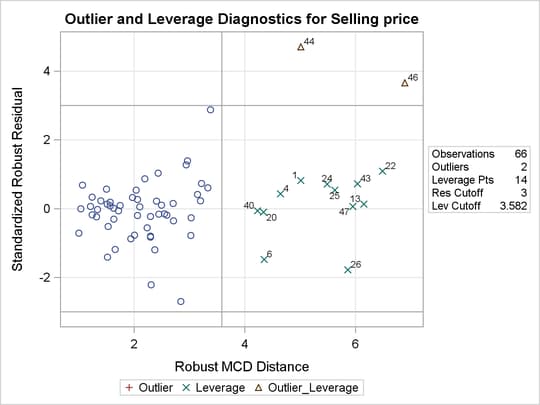
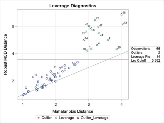
You might speculate that the projected MD and projected RD are equal to the regular MD and RD on the same data set without the variable cor. In fact, this is not true. (See Output 75.5.8 and Output 75.5.9 for the RDPLOT and DDPLOT on the data set without cor.) When included in the MODEL, cor is dropped in the distance calculation, but it is still used for the initial orthonormalization step and the  -subset searching. In this example, inclusion of cor causes all the other covariates to be centered separately for corner houses and non-corner houses. However, without cor, the centering process does not distinguish corner houses from non-corner houses, so that the MCD algorithm can still be influenced by cor through the correlation between cor and other covariates. The following statements drop the variable cor and produce the RDPLOT and DDPLOT for the reduced model, which are shown in Output 75.5.8 and Output 75.5.9:
 proc robustreg data=house method=MM plots=all;
   model price= sqft age feats ne tax/leverage diagnostics;
 run;
 ods graphics off;
Copyright © SAS Institute, Inc. All Rights Reserved.