| The QUANTREG Procedure |
Example 73.2 Quantile Regression for Econometric Growth Data
This example uses a SAS data set named growth, which contains economic growth rates for countries during two time periods, 1965–1975 and 1975–1985. The data come from a study by Barro and Lee (1994) and have also been analyzed by Koenker and Machado (1999).
There are 161 observations and 15 variables in the data set. The variables, which are listed in the following table, include the national growth rates (GDP) for the two periods, 13 covariates, and a name variable (Country) for identifying the countries in one of the two periods.
Variable |
Description |
|
Country |
Country’s name and period |
|
GDP |
Annual change per capita GDP |
|
lgdp2 |
Initial per capita GDP |
|
mse2 |
Male secondary education |
|
fse2 |
Female secondary education |
|
fhe2 |
Female higher education |
|
mhe2 |
Male higher education |
|
lexp2 |
Life expectancy |
|
lintr2 |
Human capital |
|
gedy2 |
Education |
|
Iy2 |
Investment |
|
gcony2 |
Public consumption |
|
lblakp2 |
Black market premium |
|
pol2 |
Political instability |
|
ttrad2 |
Growth rate terms trade |
The goal is to study the effect of the covariates on GDP. The following statements request median regression for a preliminary exploration. They produce the results in Output 73.2.1 through Output 73.2.6.
data growth;
   length Country$ 22;
   input Country GDP lgdp2 mse2 fse2 fhe2 mhe2 lexp2 lintr2 gedy2
         Iy2 gcony2 lblakp2 pol2 ttrad2 @@;
datalines;
Algeria75          .0415 7.330 .1320 .0670 .0050 .0220 3.880 .1138 .0382
                   .1898 .0601 .3823 .0833 .1001
Algeria85          .0244 7.745 .2760 .0740 .0070 .0370 3.978 -.107 .0437
                   .3057 .0850 .9386 .0000 .0657
Argentina75        .0187 8.220 .7850 .6200 .0740 .1660 4.181 .4060 .0221
                   .1505 .0596 .1924 .3575 -.011
Argentina85        -.014 8.407 .9360 .9020 .1320 .2030 4.211 .1914 .0243
                   .1467 .0314 .3085 .7010 -.052


   ... more lines ...

Zambia75           .0120 6.989 .3760 .1190 .0130 .0420 3.757 .4388 .0339
                   .3688 .2513 .3945 .0000 -.032
Zambia85           -.046 7.109 .4200 .2740 .0110 .0270 3.854 .8812 .0477
                   .1632 .2637 .6467 .0000 -.033
Zimbabwe75         .0320 6.860 .1450 .0170 .0080 .0450 3.833 .7156 .0337
                   .2276 .0246 .1997 .0000 -.040
Zimbabwe85         -.011 7.180 .2200 .0650 .0060 .0400 3.944 .9296 .0520
                   .1559 .0518 .7862 .7161 -.024
;
ods graphics on;

proc quantreg data=growth ci=resampling
                plots=(rdplot ddplot reshistogram);
    model GDP = lgdp2 mse2 fse2 fhe2 mhe2 lexp2
                lintr2 gedy2 Iy2 gcony2 lblakp2 pol2 ttrad2
                / quantile=.5 diagnostics leverage(cutoff=8) seed=1268;
    id Country;
    test_lgdp2: test lgdp2 / lr wald;
run;

ods graphics off;
The QUANTREG procedure employs the default simplex algorithm to estimate the parameters. The MCMB resampling method is used to compute confidence limits.
Output 73.2.1 displays model information and summary statistics for the variables in the model. Six summary statistics are computed, including the median and the median absolute deviation (MAD), which are robust measures of univariate location and scale, respectively. For the variable lintr2 (Human Capital), both the mean and standard deviation are much larger than the corresponding robust measures, median and MAD. This indicates that this variable might have outliers.
Output 73.2.2 displays parameter estimates and 95 confidence limits computed with the rank method.
| Model Information | |
|---|---|
| Data Set | WORK.GROWTH |
| Dependent Variable | GDP |
| Number of Independent Variables | 13 |
| Number of Observations | 161 |
| Optimization Algorithm | Simplex |
| Method for Confidence Limits | Resampling |
| Summary Statistics | ||||||
|---|---|---|---|---|---|---|
| Variable | Q1 | Median | Q3 | Mean | Standard Deviation |
MAD |
| lgdp2 | 6.9890 | 7.7450 | 8.6080 | 7.7905 | 0.9543 | 1.1579 |
| mse2 | 0.3160 | 0.7230 | 1.2675 | 0.9666 | 0.8574 | 0.6835 |
| fse2 | 0.1270 | 0.4230 | 0.9835 | 0.7117 | 0.8331 | 0.5011 |
| fhe2 | 0.0110 | 0.0350 | 0.0890 | 0.0792 | 0.1216 | 0.0400 |
| mhe2 | 0.0400 | 0.1060 | 0.2060 | 0.1584 | 0.1752 | 0.1127 |
| lexp2 | 3.8670 | 4.0640 | 4.2430 | 4.0440 | 0.2028 | 0.2728 |
| lintr2 | 0.00160 | 0.5604 | 1.8805 | 1.4625 | 2.5491 | 1.0058 |
| gedy2 | 0.0248 | 0.0343 | 0.0466 | 0.0360 | 0.0141 | 0.0151 |
| Iy2 | 0.1396 | 0.1955 | 0.2671 | 0.2010 | 0.0877 | 0.0981 |
| gcony2 | 0.0480 | 0.0767 | 0.1276 | 0.0914 | 0.0617 | 0.0566 |
| lblakp2 | 0 | 0.0696 | 0.2407 | 0.1916 | 0.3070 | 0.1032 |
| pol2 | 0 | 0.0500 | 0.2429 | 0.1683 | 0.2409 | 0.0741 |
| ttrad2 | -0.0240 | -0.0100 | 0.00730 | -0.00570 | 0.0375 | 0.0239 |
| GDP | 0.00290 | 0.0196 | 0.0351 | 0.0191 | 0.0248 | 0.0237 |
| Parameter Estimates | |||||||
|---|---|---|---|---|---|---|---|
| Parameter | DF | Estimate | Standard Error | 95% Confidence Limits | t Value | Pr > |t| | |
| Intercept | 1 | -0.0488 | 0.0733 | -0.1937 | 0.0961 | -0.67 | 0.5065 |
| lgdp2 | 1 | -0.0269 | 0.0041 | -0.0350 | -0.0188 | -6.58 | <.0001 |
| mse2 | 1 | 0.0110 | 0.0080 | -0.0048 | 0.0269 | 1.38 | 0.1710 |
| fse2 | 1 | -0.0011 | 0.0088 | -0.0185 | 0.0162 | -0.13 | 0.8960 |
| fhe2 | 1 | 0.0148 | 0.0321 | -0.0485 | 0.0782 | 0.46 | 0.6441 |
| mhe2 | 1 | 0.0043 | 0.0268 | -0.0487 | 0.0573 | 0.16 | 0.8735 |
| lexp2 | 1 | 0.0683 | 0.0229 | 0.0232 | 0.1135 | 2.99 | 0.0033 |
| lintr2 | 1 | -0.0022 | 0.0015 | -0.0052 | 0.0008 | -1.44 | 0.1513 |
| gedy2 | 1 | -0.0508 | 0.1654 | -0.3777 | 0.2760 | -0.31 | 0.7589 |
| Iy2 | 1 | 0.0723 | 0.0248 | 0.0233 | 0.1213 | 2.92 | 0.0041 |
| gcony2 | 1 | -0.0935 | 0.0382 | -0.1690 | -0.0181 | -2.45 | 0.0154 |
| lblakp2 | 1 | -0.0269 | 0.0084 | -0.0435 | -0.0104 | -3.22 | 0.0016 |
| pol2 | 1 | -0.0301 | 0.0093 | -0.0485 | -0.0117 | -3.23 | 0.0015 |
| ttrad2 | 1 | 0.1613 | 0.0740 | 0.0149 | 0.3076 | 2.18 | 0.0310 |
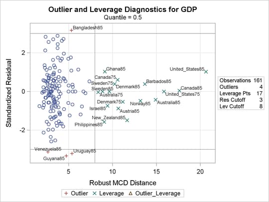
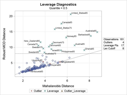
Diagnostics for the median regression fit are displayed in Output 73.2.3 and Output 73.2.4, which are requested with the PLOTS= option. Output 73.2.3 plots the standardized residuals from median regression against the robust MCD distance. This display is used to diagnose both vertical outliers and horizontal leverage points. Output 73.2.4 plots the robust MCD distance against the Mahalanobis distance. This display is used to diagnose leverage points.
The cutoff value 8 specified with the LEVERAGE option is close to the maximum of the Mahalanobis distance. Eighteen points are diagnosed as high leverage points, and almost all are countries with high human capital, which is the major contributor to the high leverage as observed from the summary statistics. Four points are diagnosed as outliers by using the default cutoff value of 3. However, these are not extreme outliers.
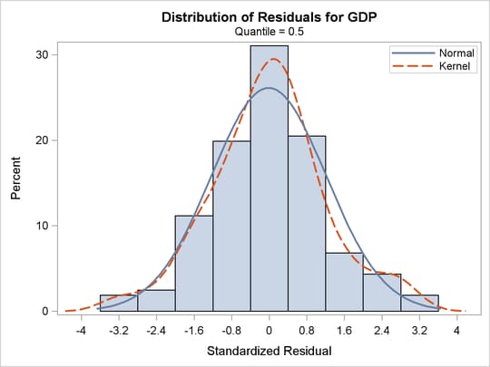
A histogram of the standardized residuals and two fitted density curves are displayed in Output 73.2.5. This shows that median regression fits the data well.
Tests of significance for the initial per-capita GDP (LGDP2) are shown in Output 73.2.6.
The QUANTREG procedure computes entire quantile processes for covariates when you specify QUANTILE=PROCESS in the MODEL statement, as follows:
ods graphics on;

proc quantreg data=growth ci=resampling;
    model GDP = lgdp2 mse2 fse2 fhe2 mhe2 lexp2 lintr2
                gedy2 Iy2 gcony2 lblakp2 pol2 ttrad2
                / quantile=process plot=quantplot seed=1268;
run;

ods graphics off;
Confidence limits for quantile processes can be computed with the sparsity or resampling methods, but not the rank method, because the computation would be prohibitively expensive.
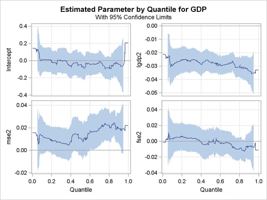
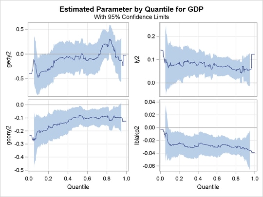
A total of 14 quantile process plots are produced. Output 73.2.7 and Output 73.2.8 display two panels of eight selected process plots. The 95 confidence bands are shaded.
Confidence Bands
Confidence Bands
As pointed out by Koenker and Machado (1999), previous studies of the Barro growth data have focused on the effect of the initial per-capita GDP on the growth of this variable (annual change per-capita GDP). A single process plot for this effect can be requested with the following statements:
ods graphics on;

proc quantreg data=growth ci=resampling;
    model GDP = lgdp2 mse2 fse2 fhe2 mhe2 lexp2 lintr2
                gedy2 Iy2 gcony2 lblakp2 pol2 ttrad2
                / quantile=process plot=quantplot(lgdp2) seed=1268;
run;

ods graphics off;
The plot is shown in Output 73.2.9.
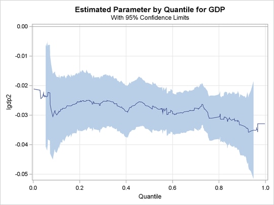
The confidence bands here are computed with the MCMB resampling method, unlike in Koenker and Machado (1999), where the rank method was used to compute confidence limits for a few selected points. Output 73.2.9 suggests that the effect of the initial level of GDP is relatively constant over the entire distribution, with a slightly stronger effect in the upper tail.
The effects of other covariates are quite varied. An interesting covariate is public consumption GDP (gcony2) (first plot in second panel), which has a constant effect over the upper half of the distribution and a larger effect in the lower tail. For an analysis of the effects of the other covariates, refer to Koenker and Machado (1999).
Copyright © SAS Institute, Inc. All Rights Reserved.