CDF Plot

For a multinomial model, the predicted cumulative distribution function is defined as

where are the indexes of the levels of the multinomial response variable, F is the CDF of the distribution used to model the cumulative probabilities, is the vector of estimated parameters, is the covariate vector, are estimated ordinal intercepts with , and is the threshold parameter, either known or estimated from the model. Let be the covariate corresponding to the dose variable and be the vector of the rest of the covariates. Let the corresponding estimated parameters be and . Then

To plot as a function of , must be specified. You can use the XDATA= option to provide the values of (see the XDATA= option in the PROC PROBIT statement for details), or use the default values that follow these rules:

• If the effect contains a continuous variable (or variables), the overall mean of this effect is used.

• If the effect is a single classification variable, the highest level of the variable is used.

The LEVEL= suboption specify the levels of the multinomial response variable for which the CDF curves are requested. There are curves for a -level multinomial response variable (for the highest level, it is the constant line 1). You can specify any of them to be plotted by the LEVEL= suboption. See the plot in Output 72.2.6 for an example.

Inverse Predicted Probability Plot

For the binomial model, the response variable is a probability. An estimate of the dose level needed for a response of is given by

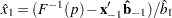where is the cumulative distribution function used to model the probability, is the vector of the rest of the covariates, is the vector of the estimated parameters corresponding to , and is the estimated parameter for the dose variable of interest.

To plot as a function of , must be specified. You can use the XDATA= option to provide the values of (see the XDATA= option in the PROC PROBIT statement for details), or use the default values that follow these rules:

• If the effect contains a continuous variable (or variables), the overall mean of this effect is used.

• If the effect is a single classification variable, the highest level of the variable is used.

Output 72.4.12 in Example 72.4 shows an inverse predicted probability plot.

Linear Predictor Plot

For both binomial models and multinomial models, the linear predictor can be plotted against the first single continuous variable (dose variable) in the MODEL statement.

Let be the covariate of the dose variable, be the vector of the rest of the covariates, be the vector of estimated parameters corresponding to , and be the estimated parameter for the dose variable of interest.

To plot as a function of , must be specified. You can use the XDATA= option to provide the values of (see the XDATA= option in the PROC PROBIT statement for details), or use the default values that follow these rules:

• If the effect contains a continuous variable (or variables), the overall mean of this effect is used.

• If the effect is a single classification variable, the highest level of the variable is used.

For the multinomial model, you can use the LEVEL= suboption to specify the levels for which the linear predictor lines are plotted.

The confidence limits for the predicted values are only available for the binomial model. Output 72.4.13 in Example 72.4 shows a linear predictor plot for a binomial model.

Predicted Probability Plot

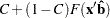
The predicted probability is

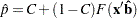for the binomial model and

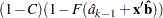for the multinomial model with response levels, where is the cumulative distribution function used to model the probability, is the vector of the covariates, are the estimated ordinal intercepts with , is the threshold parameter, either known or estimated from the model, and is the vector of estimated parameters.

To plot (or ) as a function of a continuous variable , the remaining covariates must be specified. You can use the XDATA= option to provide the values of (see the XDATA= option in the PROC PROBIT statement for details), or use the default values that follow these rules:

• If the effect contains a continuous variable (or variables), the overall mean of this effect is used.

• If the effect is a single classification variable, the highest level of the variable is used.

For the multinomial model, you can use the LEVEL= suboption to specify the levels for which the linear predictor lines are plotted.

Confidence limits are plotted only for the binomial model. Output 72.1.7 in Example 72.1 shows a predicted probability plot for a binomial model; and Output 72.2.3 in Example 72.2 shows a predicted probability plot for a multinomial model.

ODS Graph Names

PROC PROBIT assigns a name to each graph it creates using ODS. You can use these names to reference the graphs when using ODS. The names are listed in Table 72.36.

To request these graphs you must specify the ODS GRAPHICS statement in addition to the PLOTS= option described in Table 72.35. For more information about the ODS GRAPHICS statement, see Chapter 21, Statistical Graphics Using ODS.