| The NLMIXED Procedure |
Example 61.5 Failure Time and Frailty Model
In this example an accelerated failure time model with proportional hazard is fitted with and without random effects. The data are from the "Getting Started" example of PROC LIFEREG; see Chapter 48, The LIFEREG Procedure. Thirty-eight patients are divided into two groups of equal size, and different pain relievers are assigned to each group. The outcome reported is the time in minutes until headache relief. The variable censor indicates whether relief was observed during the course of the observation period (censor = 0) or whether the observation is censored (censor = 1). The SAS DATA step for these data is as follows:
data headache;
  input minutes group censor @@;
  patient = _n_;
  datalines;
11  1  0    12  1  0    19  1  0    19  1  0
19  1  0    19  1  0    21  1  0    20  1  0
21  1  0    21  1  0    20  1  0    21  1  0
20  1  0    21  1  0    25  1  0    27  1  0
30  1  0    21  1  1    24  1  1    14  2  0
16  2  0    16  2  0    21  2  0    21  2  0
23  2  0    23  2  0    23  2  0    23  2  0
25  2  1    23  2  0    24  2  0    24  2  0
26  2  1    32  2  1    30  2  1    30  2  0
32  2  1    20  2  1
;
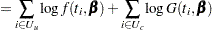
In modeling survival data, censoring of observations must be taken into account carefully. In this example, only right censoring occurs. If  ,
,  , and
, and  denote the density of failure, hazard function, and survival distribution function at time
  , respectively, the log likelihood can be written as
 |
 |
|||
 |
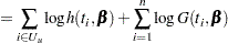 |
(See Cox and Oakes 1984, Ch. 3.) In these expressions  is the set of uncensored observations,
  is the set of censored observations, and
  denotes the total sample size.
The proportional hazards specification expresses the hazard in terms of a baseline hazard, multiplied by a constant. In this example the hazard is that of a Weibull model and is parameterized as  and
and  .
.
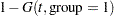
The linear predictor is set equal to the intercept in the reference group (group = 2); this defines the baseline hazard. The corresponding distribution of survival past time is 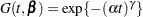 . See Cox and Oakes (1984, Table 2.1) and the section "Supported Distributions" in
Chapter 48,
The LIFEREG Procedure,
for this and other survival distribution models and various parameterizations.
. See Cox and Oakes (1984, Table 2.1) and the section "Supported Distributions" in
Chapter 48,
The LIFEREG Procedure,
for this and other survival distribution models and various parameterizations.
The following NLMIXED statements fit this accelerated failure time model and estimate the cumulative distribution function of time to headache relief:
proc nlmixed data=headache;
    bounds gamma > 0;
    linp  = b0 - b1*(group-2);
    alpha = exp(-linp);
    G_t   = exp(-(alpha*minutes)**gamma);
    g     = gamma*alpha*((alpha*minutes)**(gamma-1))*G_t;
    ll    = (censor=0)*log(g) + (censor=1)*log(G_t);
    model minutes ~ general(ll);
    predict 1-G_t out=cdf;
run;
The "Specifications" table shows that no integration is required, since the model does not contain random effects (Output 61.5.1).
No starting values were given for the three parameters. The NLMIXED procedure assigns the default value of 1.0 in this case. The negative log likelihood based on these starting values is shown in Output 61.5.2.
| Iteration History | ||||||
|---|---|---|---|---|---|---|
| Iter | Calls | NegLogLike | Diff | MaxGrad | Slope | |
| 1 | 2 | 169.244311 | 94.74602 | 22.5599 | -2230.83 | |
| 2 | 4 | 142.873508 | 26.3708 | 14.88631 | -3.64643 | |
| 3 | 6 | 140.633695 | 2.239814 | 11.25234 | -9.49454 | |
| 4 | 8 | 122.890659 | 17.74304 | 19.44959 | -2.50807 | |
| 5 | 9 | 121.396959 | 1.493699 | 13.85584 | -4.55427 | |
| 6 | 11 | 120.623843 | 0.773116 | 13.67062 | -1.38064 | |
| 7 | 12 | 119.278196 | 1.345647 | 15.78014 | -1.69072 | |
| 8 | 14 | 116.271325 | 3.006871 | 26.94029 | -3.2529 | |
| 9 | 16 | 109.427401 | 6.843925 | 19.88382 | -6.9289 | |
| 10 | 19 | 103.298102 | 6.129298 | 12.15647 | -4.96054 | |
| 11 | 22 | 101.686239 | 1.611863 | 14.24868 | -4.34059 | |
| 12 | 23 | 100.027875 | 1.658364 | 11.69853 | -13.2049 | |
| 13 | 26 | 99.9189048 | 0.108971 | 3.602552 | -0.55176 | |
| 14 | 28 | 99.8738836 | 0.045021 | 0.170712 | -0.16645 | |
| 15 | 30 | 99.8736392 | 0.000244 | 0.050822 | -0.00041 | |
| 16 | 32 | 99.8736351 | 4.071E-6 | 0.000705 | -6.9E-6 | |
| 17 | 34 | 99.8736351 | 6.1E-10 | 4.768E-6 | -1.23E-9 | |
The "Iteration History" table shows that the procedure converges after 17 iterations and 34 evaluations of the objective function (Output 61.5.3).
The parameter estimates and their standard errors shown in Output 61.5.4 are identical to those obtained with the LIFEREG procedure and the following statements:
proc lifereg data=headache;
   class group;
   model minutes*censor(1) = group / dist=weibull;
   output out=new cdf=prob;
run;
The t statistic and confidence limits are based on 38 degrees of freedom. The LIFEREG procedure computes z intervals for the parameter estimates.
For the two groups you obtain
 |
 |
|||
 |
 |
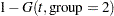
The probabilities of headache relief by minutes are estimated as
 |
 |
|||
 |
 |
These probabilities, calculated at the observed times, are shown for the two groups in Output 61.5.5 and printed with the following statements:
proc print data=cdf;
   var group censor patient minutes pred;
run;
Since the slope estimate is negative with p-value of 0.0185, you can infer that pain reliever 1 leads to overall significantly faster relief, but the estimated probabilities give no information about patient-to-patient variation within and between groups. For example, while pain reliever 1 provides faster relief overall, some patients in group 2 might respond more quickly than some patients in group 1. A frailty model enables you to accommodate and estimate patient-to-patient variation in health status by introducing random effects into a subject’s hazard function.
| Obs | group | censor | patient | minutes | Pred |
|---|---|---|---|---|---|
| 1 | 1 | 0 | 1 | 11 | 0.03336 |
| 2 | 1 | 0 | 2 | 12 | 0.04985 |
| 3 | 1 | 0 | 3 | 19 | 0.35975 |
| 4 | 1 | 0 | 4 | 19 | 0.35975 |
| 5 | 1 | 0 | 5 | 19 | 0.35975 |
| 6 | 1 | 0 | 6 | 19 | 0.35975 |
| 7 | 1 | 0 | 7 | 21 | 0.51063 |
| 8 | 1 | 0 | 8 | 20 | 0.43325 |
| 9 | 1 | 0 | 9 | 21 | 0.51063 |
| 10 | 1 | 0 | 10 | 21 | 0.51063 |
| 11 | 1 | 0 | 11 | 20 | 0.43325 |
| 12 | 1 | 0 | 12 | 21 | 0.51063 |
| 13 | 1 | 0 | 13 | 20 | 0.43325 |
| 14 | 1 | 0 | 14 | 21 | 0.51063 |
| 15 | 1 | 0 | 15 | 25 | 0.80315 |
| 16 | 1 | 0 | 16 | 27 | 0.90328 |
| 17 | 1 | 0 | 17 | 30 | 0.97846 |
| 18 | 1 | 1 | 18 | 21 | 0.51063 |
| 19 | 1 | 1 | 19 | 24 | 0.73838 |
| 20 | 2 | 0 | 20 | 14 | 0.04163 |
| 21 | 2 | 0 | 21 | 16 | 0.07667 |
| 22 | 2 | 0 | 22 | 16 | 0.07667 |
| 23 | 2 | 0 | 23 | 21 | 0.24976 |
| 24 | 2 | 0 | 24 | 21 | 0.24976 |
| 25 | 2 | 0 | 25 | 23 | 0.35674 |
| 26 | 2 | 0 | 26 | 23 | 0.35674 |
| 27 | 2 | 0 | 27 | 23 | 0.35674 |
| 28 | 2 | 0 | 28 | 23 | 0.35674 |
| 29 | 2 | 1 | 29 | 25 | 0.47982 |
| 30 | 2 | 0 | 30 | 23 | 0.35674 |
| 31 | 2 | 0 | 31 | 24 | 0.41678 |
| 32 | 2 | 0 | 32 | 24 | 0.41678 |
| 33 | 2 | 1 | 33 | 26 | 0.54446 |
| 34 | 2 | 1 | 34 | 32 | 0.87656 |
| 35 | 2 | 1 | 35 | 30 | 0.78633 |
| 36 | 2 | 0 | 36 | 30 | 0.78633 |
| 37 | 2 | 1 | 37 | 32 | 0.87656 |
| 38 | 2 | 1 | 38 | 20 | 0.20414 |
The following statements model the hazard for patient  in terms of
 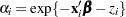 , where
  is a (normal) random patient effect. Notice that the only difference from the previous NLMIXED statements are the RANDOM statement and the addition of z in the linear predictor. The empirical Bayes estimates of the random effect (RANDOM statement), the parameter estimates (ODS OUTPUT statement), and the estimated cumulative distribution function (PREDICT statement) are saved to subsequently graph the patient-specific distribution functions.
ods output ParameterEstimates=est;
proc nlmixed data=headache;
    bounds gamma > 0;
    linp  = b0 - b1*(group-2) + z;
    alpha = exp(-linp);
    G_t   = exp(-(alpha*minutes)**gamma);
    g     = gamma*alpha*((alpha*minutes)**(gamma-1))*G_t;
    ll = (censor=0)*log(g) + (censor=1)*log(G_t);
    model minutes ~ general(ll);
    random z ~ normal(0,exp(2*logsig)) subject=patient out=EB;
    predict 1-G_t out=cdf;
run;
| Specifications | |
|---|---|
| Data Set | WORK.HEADACHE |
| Dependent Variable | minutes |
| Distribution for Dependent Variable | General |
| Random Effects | z |
| Distribution for Random Effects | Normal |
| Subject Variable | patient |
| Optimization Technique | Dual Quasi-Newton |
| Integration Method | Adaptive Gaussian Quadrature |
The "Specifications" table shows that the objective function is computed by adaptive Gaussian quadrature because of the presence of random effects (compare Output 61.5.6 and Output 61.5.1). The "Dimensions" table reports that nine quadrature points are being used to integrate over the random effects (Output 61.5.7).
| Iteration History | ||||||
|---|---|---|---|---|---|---|
| Iter | Calls | NegLogLike | Diff | MaxGrad | Slope | |
| 1 | 5 | 142.121411 | 28.82225 | 12.14484 | -88.8664 | |
| 2 | 7 | 136.440369 | 5.681042 | 25.93096 | -65.7217 | |
| 3 | 9 | 122.972041 | 13.46833 | 46.56546 | -146.887 | |
| 4 | 11 | 120.904825 | 2.067216 | 23.77936 | -94.2862 | |
| 5 | 13 | 109.224144 | 11.68068 | 57.65493 | -92.4075 | |
| 6 | 15 | 105.064733 | 4.159411 | 4.824649 | -19.5879 | |
| 7 | 16 | 101.902207 | 3.162526 | 14.1287 | -6.33767 | |
| 8 | 18 | 99.6907395 | 2.211468 | 7.676822 | -3.42364 | |
| 9 | 20 | 99.3654033 | 0.325336 | 5.689204 | -0.93978 | |
| 10 | 22 | 99.2602178 | 0.105185 | 0.317643 | -0.23408 | |
| 11 | 24 | 99.254434 | 0.005784 | 1.17351 | -0.00556 | |
| 12 | 25 | 99.2456973 | 0.008737 | 0.247412 | -0.00871 | |
| 13 | 27 | 99.2445445 | 0.001153 | 0.104942 | -0.00218 | |
| 14 | 29 | 99.2444958 | 0.000049 | 0.005646 | -0.0001 | |
| 15 | 31 | 99.2444957 | 9.147E-8 | 0.000271 | -1.84E-7 | |
The procedure converges after 15 iterations (Output 61.5.8). The achieved  log likelihood is only 1.2 less than that in the model without random effects (compare Output 61.5.9 and Output 61.5.4). Compared to a chi-square distribution with one degree of freedom, the addition of the random effect appears not to improve the model significantly. You must exercise care, however, in interpreting likelihood ratio tests when the value under the null hypothesis falls on the boundary of the parameter space (see, for example, Self and Liang 1987).
| Parameter Estimates | |||||||||
|---|---|---|---|---|---|---|---|---|---|
| Parameter | Estimate | Standard Error | DF | t Value | Pr > |t| | Alpha | Lower | Upper | Gradient |
| gamma | 6.2867 | 2.1334 | 37 | 2.95 | 0.0055 | 0.05 | 1.9641 | 10.6093 | -1.89E-7 |
| b0 | 3.2786 | 0.06576 | 37 | 49.86 | <.0001 | 0.05 | 3.1453 | 3.4118 | 0.000271 |
| b1 | -0.1761 | 0.08264 | 37 | -2.13 | 0.0398 | 0.05 | -0.3436 | -0.00868 | 0.000111 |
| logsig | -1.9027 | 0.5273 | 37 | -3.61 | 0.0009 | 0.05 | -2.9711 | -0.8343 | 0.000027 |
The estimate of the Weibull parameter has changed drastically from the model without random effects (compare Output 61.5.10 and Output 61.5.4). The variance of the patient random effect is  . The listing in Output 61.5.11 shows the empirical Bayes estimates of the random effects. These are the adjustments made to the linear predictor in order to obtain a patient’s survival distribution. The listing is produced with the following statements:
proc print data=eb;
   var Patient Effect Estimate StdErrPred;
run;
| Obs | patient | Effect | Estimate | StdErrPred |
|---|---|---|---|---|
| 1 | 1 | z | -0.13597 | 0.23249 |
| 2 | 2 | z | -0.13323 | 0.22793 |
| 3 | 3 | z | -0.06294 | 0.13813 |
| 4 | 4 | z | -0.06294 | 0.13813 |
| 5 | 5 | z | -0.06294 | 0.13813 |
| 6 | 6 | z | -0.06294 | 0.13813 |
| 7 | 7 | z | -0.02568 | 0.11759 |
| 8 | 8 | z | -0.04499 | 0.12618 |
| 9 | 9 | z | -0.02568 | 0.11759 |
| 10 | 10 | z | -0.02568 | 0.11759 |
| 11 | 11 | z | -0.04499 | 0.12618 |
| 12 | 12 | z | -0.02568 | 0.11759 |
| 13 | 13 | z | -0.04499 | 0.12618 |
| 14 | 14 | z | -0.02568 | 0.11759 |
| 15 | 15 | z | 0.05980 | 0.11618 |
| 16 | 16 | z | 0.10458 | 0.12684 |
| 17 | 17 | z | 0.17147 | 0.14550 |
| 18 | 18 | z | 0.06471 | 0.13807 |
| 19 | 19 | z | 0.11157 | 0.14604 |
| 20 | 20 | z | -0.13406 | 0.22899 |
| 21 | 21 | z | -0.12698 | 0.21667 |
| 22 | 22 | z | -0.12698 | 0.21667 |
| 23 | 23 | z | -0.08506 | 0.15701 |
| 24 | 24 | z | -0.08506 | 0.15701 |
| 25 | 25 | z | -0.05797 | 0.13294 |
| 26 | 26 | z | -0.05797 | 0.13294 |
| 27 | 27 | z | -0.05797 | 0.13294 |
| 28 | 28 | z | -0.05797 | 0.13294 |
| 29 | 29 | z | 0.06420 | 0.13956 |
| 30 | 30 | z | -0.05797 | 0.13294 |
| 31 | 31 | z | -0.04266 | 0.12390 |
| 32 | 32 | z | -0.04266 | 0.12390 |
| 33 | 33 | z | 0.07618 | 0.14132 |
| 34 | 34 | z | 0.16292 | 0.16460 |
| 35 | 35 | z | 0.13193 | 0.15528 |
| 36 | 36 | z | 0.06327 | 0.12124 |
| 37 | 37 | z | 0.16292 | 0.16460 |
| 38 | 38 | z | 0.02074 | 0.14160 |
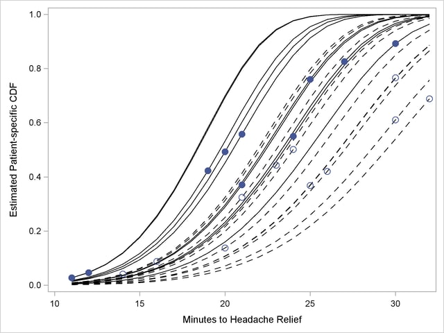
The predicted values and patient-specific survival distributions can be plotted with the SAS code that follows:
proc transpose data=est(keep=estimate)
    out=trest(rename=(col1=gamma col2=b0 col3=b1));
run;

data pred;
   merge eb(keep=estimate) headache(keep=patient group);
    array pp{2} pred1-pred2;
    if _n_ = 1 then set trest(keep=gamma b0 b1);
    do time=11 to 32;
      linp      = b0 - b1*(group-2) + estimate;
      pp{group} = 1-exp(- (exp(-linp)*time)**gamma);
      symbolid  = patient+1;
      output;
    end;
    keep pred1 pred2 time patient;
run;

data pred;
   merge pred
         cdf(where  = (group=1)
             rename = (pred=pcdf1 minutes=minutes1)
             keep   = pred minutes group)
         cdf(where  = (group=2)
             rename = (pred=pcdf2 minutes=minutes2)
             keep   = pred minutes group);
   drop group;
run;

proc sgplot data=pred noautolegend;
   label minutes1='Minutes to Headache Relief'
         pcdf1   ='Estimated Patient-specific CDF';
   series  x=time     y=pred1  /
           group=patient
           lineattrs=(pattern=solid color=black);
   series  x=time     y=pred2  /
           group=patient
           lineattrs=(pattern=dash color=black);
   scatter x=minutes1 y=pcdf1  /
           markerattrs=(symbol=CircleFilled size=9);
   scatter x=minutes2 y=pcdf2  /
           markerattrs=(symbol=Circle       size=9);
run;
The separation of the distribution functions by groups is evident in Output 61.5.12. Most of the distributions of patients in the first group are to the left of the distributions in the second group. The separation is not complete, however. Several patients who are assigned the second pain reliever experience headache relief more quickly than patients assigned to the first group.
Copyright © SAS Institute, Inc. All Rights Reserved.