Example 52.12 Using a Transformation to Improve Mixing

Proper transformations of parameters can often improve the mixing in PROC MCMC. You already saw this in Nonlinear Poisson Regression Models, which sampled using the scale of parameters that priors that are strictly positive, such as the gamma priors. This example shows another useful transformation: the logit transformation on parameters that take a uniform prior on [0, 1].

The data set is taken from Sharples (1990). It is used in Chaloner and Brant (1988) and Chaloner (1994) to identify outliers in the data set in a two-level hierarchical model. Congdon (2003) also uses this data set to demonstrates the same technique. This example uses the data set to illustrate how mixing can be improved using transformation and does not address the question of outlier detection as in those papers. The following statements create the data set:

data inputdata;
   input nobs grp y @@;
   ind = _n_;
   datalines;
1 1 24.80 2 1 26.90 3 1 26.65
4 1 30.93 5 1 33.77 6 1 63.31
1 2 23.96 2 2 28.92 3 2 28.19
4 2 26.16 5 2 21.34 6 2 29.46
1 3 18.30 2 3 23.67 3 3 14.47
4 3 24.45 5 3 24.89 6 3 28.95
1 4 51.42 2 4 27.97 3 4 24.76
4 4 26.67 5 4 17.58 6 4 24.29
1 5 34.12 2 5 46.87 3 5 58.59
4 5 38.11 5 5 47.59 6 5 44.67
;

There are five groups (grp, ) with six observations (nobs, ) in each. The two-level hierarchical model is specified as follows:

with the precision parameters related to each other in the following way:

The total number of parameters in this model is eight: , and .

The following statements fit the model:

ods graphics on;
proc mcmc data=inputdata nmc=50000 thin=10 outpost=m1 seed=17
          plot=trace;
   ods select ess tracepanel;
   array theta[5];
 
   parms theta:;
   parms p tau;
   parms mu ;
 
   beginnodata;
   hyper p ~ uniform(0,1);
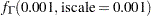
   hyper tau ~ gamma(shape=0.001,iscale=0.001);
   hyper mu ~ normal(0,prec=0.00000001);
   taub = tau/p;
   prior theta: ~ normal(mu,prec=taub);
   tauw = taub-tau;
   endnodata;
 
   model y ~ normal(theta[grp],prec=tauw);
run;

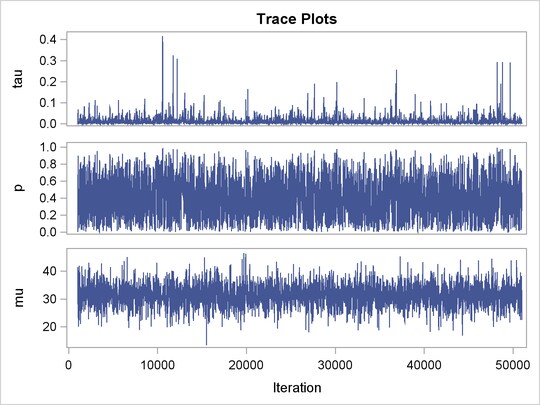
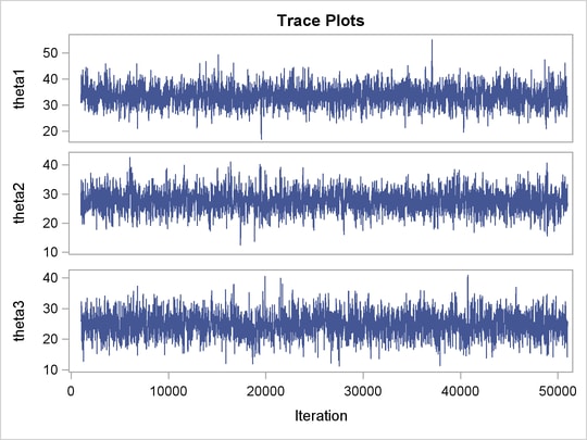
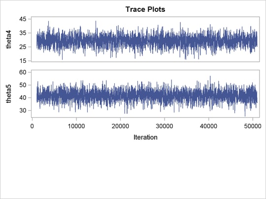
The ODS SELECT statement displays the effective sample size table and the trace plots. The ODS GRAPHICS ON statement requests ODS Graphics. The PROC MCMC statement specifies the usual options for the MCMC run and produces trace plots (PLOTS=TRACE). The ARRAY statement allocates an array of size 5 for theta. The three PARMS statements put parameters in three different blocks. The remaining statements specify the hyperprior, prior, and likelihood for the data, as described previously. The resulting trace plots are shown in Output 52.12.1, and the effective sample sizes table is shown in Output 52.12.2.

Output 52.12.1 Trace Plots

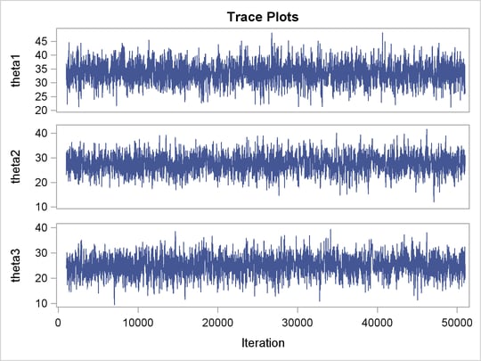
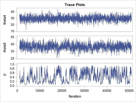
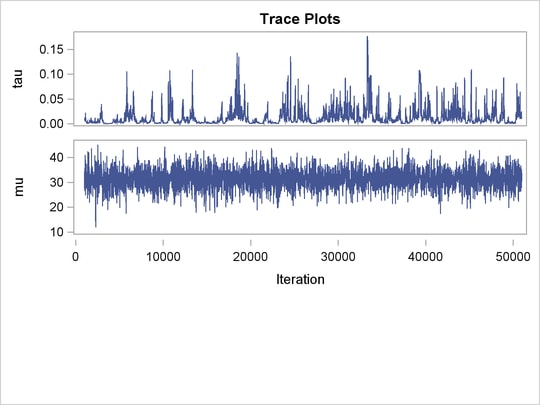
The trace plots show that most parameters have relatively good mixing. Two exceptions appear to be and . The trace plot of shows a slow periodic movement. The parameter does not have good mixing either. When the values are close to zero, the chain stands there for long periods of time. An inspection of the effective sample sizes table reveals the same conclusion: and have much smaller ESSs than the rest of the parameters.

A scatter plot of the posterior samples of and reveals why mixing is bad in these two dimensions. The following statements generate the scatter plot in Output 52.12.3:

title 'Scatter Plot of Parameters on Original Scales';
 
proc sgplot data=m1;
   yaxis label = 'p';
   xaxis label = 'tau' values=(0 to 0.4 by 0.1);
   scatter x = tau y = p;
run;

Output 52.12.3 Scatter Plot of versus

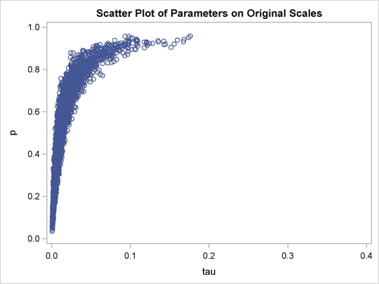
The two parameters clearly have a nonlinear relationship. It is not surprising that the Metropolis algorithm does not work well here. The algorithm is designed for cases where the parameters are linearly related with each other.

Instead of sampling on , you can sample on the log of . The formulation

where and are density functions for the gamma and egamma distributions. See the section Standard Distributions for the definitions of the distributions. In addition, you can sample on the logit of . The formulation

is equivalent to the following transformation:

The following statements fit the same model by using transformed parameters:

proc mcmc data=inputdata nmc=50000 thin=10 outpost=m2 seed=17
          monitor=(tau p mu theta) plot=trace;
   ods select ess tracepanel;
   array theta[5];
 
   parms theta:;
   parms lgp 0 ltau ;
   parms mu ;
 
   beginnodata;
   prior ltau ~ egamma(shape=0.001,iscale=0.001);
   lp = -lgp - 2*log(1+exp(-lgp));
   prior lgp ~ general(lp);
   tau = exp(ltau);
   p = (1+exp(-lgp))**-1;
   prior mu ~ normal(0,prec=0.00000001);
   taub = tau/p;
   prior theta: ~ normal(mu,prec=taub);
   tauw = taub-tau;
   endnodata;
 
   model y ~ normal(theta[grp],prec=tauw);
run;
ods graphics off;

The variable lgp is the logit transformation of , and ltau is the log transformation of . The prior for ltau is egamma. The lp assignment statement evaluates the log density of . The tau and p assignment statements transform the parameters back to their original scales. The prior distributions for mu, theta, and the log likelihood in the MODEL statement remain unchanged. Trace plots (Output 52.12.4) and effective sample size (Output 52.12.5) both show significant improvements in the mixing for both and .

Output 52.12.4 Trace Plots after Transformation

The following statements generate Output 52.12.6 and Output 52.12.7:

title 'Scatter Plot of Parameters on Transformed Scales';
 
proc sgplot data=m2;
   yaxis label = 'logit(p)';
   xaxis label = 'log(tau)';
   scatter x = ltau y = lgp;
run;
 
title 'Scatter Plot of Parameters on Original Scales';
 
proc sgplot data=m2;
   yaxis label = 'p';
   xaxis label = 'tau';
   scatter x = tau y = p;
run;

Output 52.12.6 Scatter Plot of versus , After Transformation

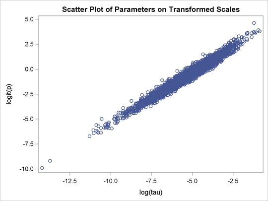
Output 52.12.7 Scatter Plot of versus , After Transformation

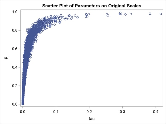
The scatter plot of versus shows a linear relationship between the two transformed parameters, and this explains the improvement in mixing. In addition, the transformations also help the Markov chain better explore in the original parameter space. Output 52.12.7 shows a scatter plot of versus . The plot is similar to Output 52.12.3. However, note that tau has a far longer tail in Output 52.12.7, extending all the way to 0.4 as opposed to 0.15 in Output 52.12.3. This means that the second Markov chain can explore this dimension of the parameter more efficiently, and as a result, you are able to draw more precise inference with an equal number of simulations.