PROC LOGISTIC: Regression Diagnostics :: SAS/STAT(R) 9.22 User's Guide

The LOGISTIC Procedure

Regression Diagnostics

For binary response data, regression diagnostics developed by Pregibon (1981) can be requested by specifying the INFLUENCE option. For diagnostics available with conditional logistic regression, see the section Regression Diagnostic Details. These diagnostics can also be obtained from the OUTPUT statement.

This section uses the following notation:

$\text{[math]}$: $\text{[math]}$ is the number of event responses out of $\text{[math]}$ trials for the $\text{[math]}$ th observation. If events/trials syntax is used, $\text{[math]}$ is the value of events and $\text{[math]}$ is the value of trials. For single-trial syntax, $\text{[math]}$ , and $\text{[math]}$ if the ordered response is 1, and $\text{[math]}$ if the ordered response is 2.
$\text{[math]}$: is the weight of the $\text{[math]}$ th observation.
$\text{[math]}$: is the probability of an event response for the $\text{[math]}$ th observation given by 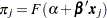$\text{[math]}$ , where $\text{[math]}$ is the inverse link function.
$\text{[math]}$: is the maximum likelihood estimate (MLE) of $\text{[math]}$ .
$\text{[math]}$: is the estimated covariance matrix of $\text{[math]}$ .
$\text{[math]}$: $\text{[math]}$ is the estimate of $\text{[math]}$ evaluated at $\text{[math]}$ , and $\text{[math]}$ .

Pregibon (1981) suggests using the index plots of several diagnostic statistics to identify influential observations and to quantify the effects on various aspects of the maximum likelihood fit. In an index plot, the diagnostic statistic is plotted against the observation number. In general, the distributions of these diagnostic statistics are not known, so cutoff values cannot be given for determining when the values are large. However, the IPLOTS and INFLUENCE options in the MODEL statement and the PLOTS option in the PROC LOGISTIC statement provide displays of the diagnostic values, allowing visual inspection and comparison of the values across observations. In these plots, if the model is correctly specified and fits all observations well, then no extreme points should appear.

The next five sections give formulas for these diagnostic statistics.

Hat Matrix Diagonal (Leverage)

The diagonal elements of the hat matrix are useful in detecting extreme points in the design space where they tend to have larger values. The $\text{[math]}$ th diagonal element is

$\text{[math]}$

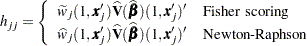where

	$\text{[math]}$	$\text{[math]}$	$\text{[math]}$
	$\text{[math]}$	$\text{[math]}$	$\text{[math]}$

and $\text{[math]}$ and $\text{[math]}$ are the first and second derivatives of the link function $\text{[math]}$ , respectively.

For a binary response logit model, the hat matrix diagonal elements are

$\text{[math]}$

If the estimated probability is extreme (less than 0.1 and greater than 0.9, approximately), then the hat diagonal might be greatly reduced in value. Consequently, when an observation has a very large or very small estimated probability, its hat diagonal value is not a good indicator of the observation’s distance from the design space (Hosmer and Lemeshow; 2000, p. 171).

Pearson Residuals and Deviance Residuals

Pearson and deviance residuals are useful in identifying observations that are not explained well by the model. Pearson residuals are components of the Pearson chi-square statistic and deviance residuals are components of the deviance. The Pearson residual for the $\text{[math]}$ th observation is

$\text{[math]}$

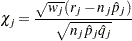The Pearson chi-square statistic is the sum of squares of the Pearson residuals.

The deviance residual for the $\text{[math]}$ th observation is

$\text{[math]}$

where the plus (minus) in $\text{[math]}$ is used if $\text{[math]}$ is greater (less) than $\text{[math]}$ . The deviance is the sum of squares of the deviance residuals.

DFBETAS

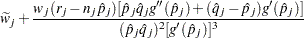
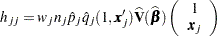
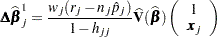
For each parameter estimate, the procedure calculates a DFBETAS diagnostic for each observation. The DFBETAS diagnostic for an observation is the standardized difference in the parameter estimate due to deleting the observation, and it can be used to assess the effect of an individual observation on each estimated parameter of the fitted model. Instead of reestimating the parameter every time an observation is deleted, PROC LOGISTIC uses the one-step estimate. See the section Predicted Probability of an Event for Classification. For the $\text{[math]}$ th observation, the DFBETAS are given by

$\text{[math]}$

where $\text{[math]}$ is the standard error of the $\text{[math]}$ th component of $\text{[math]}$ , and $\text{[math]}$ is the $\text{[math]}$ th component of the one-step difference

$\text{[math]}$

$\text{[math]}$ is the approximate change ( $\text{[math]}$ ) in the vector of parameter estimates due to the omission of the $\text{[math]}$ th observation. The DFBETAS are useful in detecting observations that are causing instability in the selected coefficients.

C and CBAR

C and CBAR are confidence interval displacement diagnostics that provide scalar measures of the influence of individual observations on $\text{[math]}$ . These diagnostics are based on the same idea as the Cook distance in linear regression theory (Cook and Weisberg; 1982), but use the one-step estimate. C and CBAR for the $\text{[math]}$ th observation are computed as

$\text{[math]}$

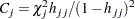and

$\text{[math]}$

respectively.

Typically, to use these statistics, you plot them against an index and look for outliers.

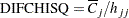
DIFDEV and DIFCHISQ

DIFDEV and DIFCHISQ are diagnostics for detecting ill-fitted observations; in other words, observations that contribute heavily to the disagreement between the data and the predicted values of the fitted model. DIFDEV is the change in the deviance due to deleting an individual observation while DIFCHISQ is the change in the Pearson chi-square statistic for the same deletion. By using the one-step estimate, DIFDEV and DIFCHISQ for the $\text{[math]}$ th observation are computed as

$\text{[math]}$

and

$\text{[math]}$

Top of Page