PROC KDE: Changing the Bandwidth (Bivariate) :: SAS/STAT(R) 9.22 User's Guide

The KDE Procedure

Example 45.3 Changing the Bandwidth (Bivariate)

Recall the analysis from the section Getting Started: KDE Procedure. Suppose you would like a slightly smoother estimate. You could then rerun the analysis with a larger bandwidth:

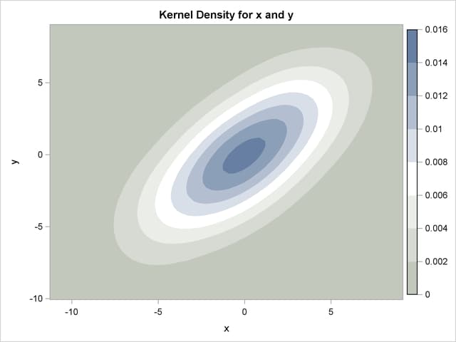
ods graphics on;
proc kde data=bivnormal;
   bivar x y / bwm=2;
run;

The BWM= option requests bandwidth multipliers of 2 for both x and y. With ODS Graphics enabled, the BIVAR statement produces a contour plot, as shown in Output 45.3.1.

Output 45.3.1 Contour Plot of Estimated Density with Additional Smoothing

Multiple Bandwidths

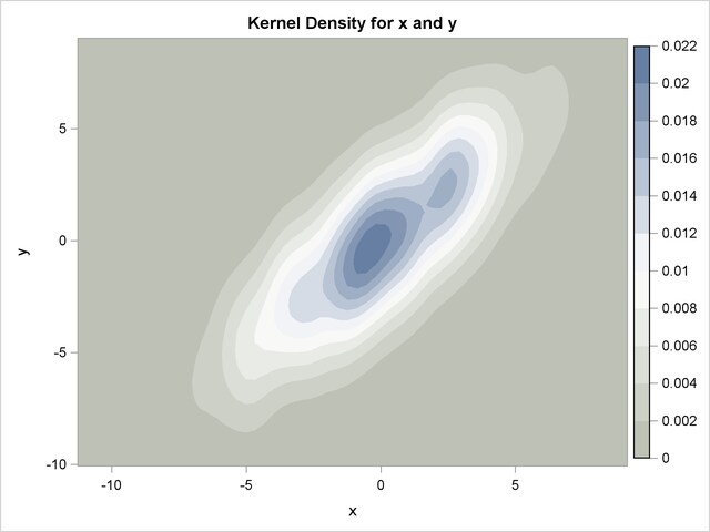
You can also specify multiple bandwidths with only one run of the KDE procedure. Notice that by specifying pairs of variables inside parentheses, a kernel density estimate is computed for each pair. In the following statements the first kernel density is computed with the default bandwidth, but the second kernel density specifies a bandwidth multiplier of 0.5 for the variable x and a multiplier of 2 for the variable y:

proc kde data=bivnormal;
   bivar (x y) (x (bwm=0.5) y (bwm=2));
run;
ods graphics off;

The contour plot of the second kernel density estimate is shown in Output 45.3.2.

Output 45.3.2 Contour Plot of Estimated Density with Different Smoothing for x and y

Top of Page